Superior web optimization Audit Strategies: Excel

Making ready and dealing with knowledge takes a little bit work, however you’ll be an ol’ professional very quickly with a little bit follow. It truly is quite a bit simpler than you assume.

If you wish to breeze by way of knowledge preparation effortlessly, obtain The Full Technical web optimization Audit Workbook.

Ideas For Cleansing And Making ready Information

One of many first challenges can be cleansing the info.

In different phrases, you’ll have to take away empty rows or columns that may mess up your knowledge, label all of the columns accurately, and standardize the info (e.g., you might have “AZ” in a single knowledge set, however “Arizona” in one other knowledge set. They have to be the identical in order that Excel or Google Sheets can acknowledge that they’re the identical.)

Cleansing knowledge is a ache, however there are some methods that may make it sooner.

How To Discover And Take away Empty Rows

Google Sheets and Excel primarily work the identical solution to take away blanks. It’s simply that the instructions look a little bit totally different.

In Excel:

1. Choose the entire knowledge.
2. Click on House > Discover & Choose > Go To Particular, choose “Blanks,” and click on “OK.”
3. Proper-click on a particular cell and choose “Delete” from the dropdown menu.
4. Select “Complete row” and click on “OK.”

In Google Sheets:

1. Choose the info.
2. Click on Information > Filter and uncheck the field subsequent to “Blanks.”
3. Then, choose “Create a filter” within the Information tab.
4. Click on the filter icon in row 1. Then, Clear > Blanks.
5. Ctrl (or Cmd) + A and delete rows.
6. Flip off the filter (Information tab > Flip off filter).

How To Discover And Take away Empty Columns

The steps to take away empty columns are primarily the identical as eradicating empty rows. Skip this step, nonetheless, and also you’ll discover that knowledge evaluation abruptly entails a number of errors.

In Excel:

1. Choose knowledge.
2. Click on House > Discover & Choose > Go To Particular > Blanks, and click on “OK.”
3. Use Ctrl (or Cmd) + Spacebar to pick your complete column and click on Delete within the right-click menu.
4. Choose “Complete column” and click on “OK.”

In Google Sheets:

1. Choose the info.
2. Click on Information > Filter.
3. Click on the filter button in row 1 and uncheck the field subsequent to “Blanks.”
4. Choose the empty columns, right-click, and choose “Delete column” from the menu.

How To Use Concatenate To Mix Two Cells

You possibly can mix textual content right into a single cell utilizing the CONCATENATE operate.

It’s significantly helpful for combining first and final names, dates, or different knowledge which might be introduced to you in a number of columns. And by chaining them collectively, you may manage and merge knowledge right into a single sheet.

In Excel and Google Sheets:

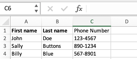
Let’s faux we have now two knowledge units in separate sheets:

Sheet 1 has first identify, final identify, and electronic mail.

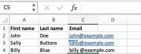
Sheet 2 has first identify, final identify, and cellphone quantity.

Let’s mix the info from the 2 sheets to make the info simpler to work with.

First, let’s mix first and final names in case we have now a couple of John in our dataset.

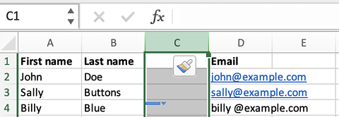
1. Insert a brand new column in Sheets 1 and a couple of to the best of the “final identify” column.

2. In C2 on each sheets, enter the method:

=CONCATENATE(A2," ",B2)

(This says, for the string in A2, depart an area (” “) after which add the contents of B2.)

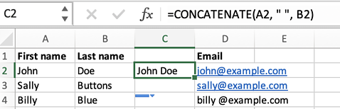
3. Choose C2, click on the underside proper nook of C2, and drag it to the underside of your knowledge to repeat the method down.

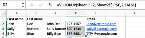
4. Now, insert a brand new column to the best of the mixed identify (C) in Sheet 1.

5. Within the first row of the brand new column, enter the next method:

=VLOOKUP(Sheet1!C2,Sheet2!$C:$E,2,FALSE)

This method will seek for no matter is in C2 in Sheet 2 (the complete identify of John Doe) and return the corresponding cellphone quantity to Sheet 1.

6. Copy the method within the first row of the brand new column in Sheet 1 and paste it into the remaining rows within the column as you probably did with the concatenate method.

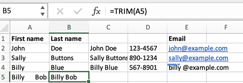
Different Fast And Useful Information Cleansing Instructions

Wish to take away undesirable area inside a cell? Use Trim. (It really works in each Excel and Google Sheets.)

How To Mix Information Units Into A Single Desk Utilizing Google Sheets

One other frequent activity you’ll end up doing when working with knowledge is getting all of it into the identical sheet.

However a phrase of warning: Combining a number of knowledge recordsdata generally is a nightmare if you happen to don’t put together your knowledge. So, make it possible for all of them have the identical construction and format earlier than you begin.

Let’s begin with one thing simple and work our manner up.

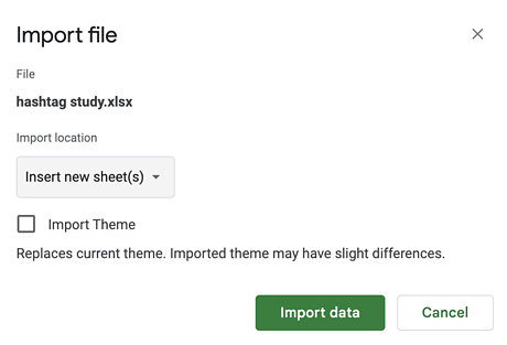
Import One Complete Dataset Into One other

Import knowledge into an present sheet. File > Import> Choose the info set to import > Insert. Then, change the dropdown to “Insert new sheet.” It would add the brand new knowledge beneath.

Use The “QUERY” Operate

Let’s say you’ve got a sheet with visitors and bounce charges, and also you need to create a sheet with bounce charges which might be beneath 50% to determine your better-performing pages.

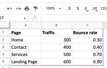
=QUERY(Sheet1!A2:C5, “SELECT A,B,C WHERE C < 0.5”)

This method will create a brand new knowledge set that features all the data for any pages assembly our requirement of a 50% bounce charge.

On this method, Sheet1!A2:C5 are the ranges it appears by way of; SELECT A,B,C tells it which cells to tug if the bounce charge is lower than 0.5; and C < 0.5” is the maths operate that tells it to solely copy the data from the opposite sheet if the worth in column C is lower than 0.5.

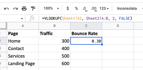
Use The “VLOOKUP” Operate

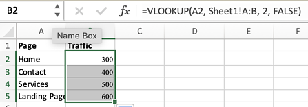
The VLOOKUP operate permits you to seek for a worth in a single knowledge set and return a corresponding worth from one other knowledge set. Right here’s an instance of find out how to use it:

Two sheets: one with bounce charges (Sheet 2) and one with visitors numbers (Sheet 1).

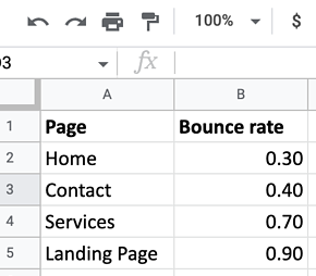
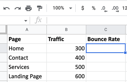
=VLOOKUP(Sheet1!A2, Sheet2!A:B, 2, FALSE)

This method will seek for the worth in Sheet1!A2 within the first column of Sheet 2 and return the corresponding worth from the second column of Sheet 2 after they match.

Your web page names have to be the identical on each sheets. In case you have a “sale web page” in a single knowledge set and a “touchdown web page” on the opposite, it gained’t work.

The “INDEX” And “MATCH” Features

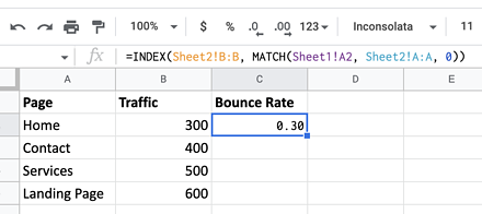
=INDEX(Sheet2!B:B, MATCH(Sheet1!A2, Sheet2!A:A, 0))

This method will seek for the worth in Sheet1!A2 within the first column of Sheet 2 and return the corresponding worth from the second column of Sheet 2.

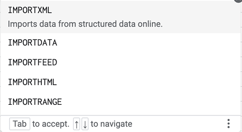
Import Features In The Components Bar

IMPORTRANGE can get the job achieved from the method bar.

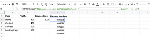
=IMPORTRANGE(“spreadsheet_url”, “range_string”)

Copy the URL for the opposite knowledge set. (Every part earlier than the # signal.)

Then, inform it what vary to repeat throughout. (It would mechanically replace as modifications are made on the opposite sheet.)

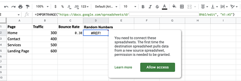
It provides you with an error, so that you simply have to provide it entry. Different import sorts you may play with?

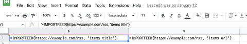
Import through RSS feed:

=IMPORTFEED(https://instance.com/rss, “objects title”)

Import through XML:

=IMPORTXML(“https://instance.com/”, “xpath_query”)

Import through on-line structured knowledge file (like a CSV):

=IMPORTDATA(“https://instance.com/file.csv”)

Import from a desk on a webpage:

=IMPORTHTML(“https://instance.com/slug”,”desk”,1)

(The place “desk” is the question and “1” is the index begin location.)

No-Components Options

Google Sheets Add-Ons can be actually useful if you happen to’d prefer to keep away from formulation. I’d encourage you to provide the formulation a strive, although. They’re versatile. (They usually make you’re feeling type of good and highly effective after they work.)

How To Mix Information Units Into A Single Desk Utilizing Excel

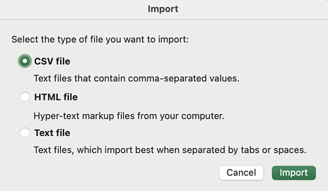
Easy Import

Select File > Import > Choose the info set. Then, inform it if it’s deliminated or a mounted width file. > Inform it how the file is delineated (tabs, colons, and so forth.). > Choose knowledge format (textual content, dates, and so forth.). > End.

Lastly, inform it if you wish to add it to an present sheet (and the place), or if it ought to create a brand new sheet.

Use Excel’s Energy Question

If you happen to cherished the question fetching in Google Sheets, you’ll love Energy Question in Excel. Exterior of Python, R, and studying a complete coding language, it’s the most helpful and highly effective characteristic you should use to work with massive knowledge units.

You’ll additionally discover glorious documentation and loads of movies (with knowledge you may obtain to comply with together with) that can assist you be taught to make use of it. Month-to-month reporting knowledge is a superb follow.

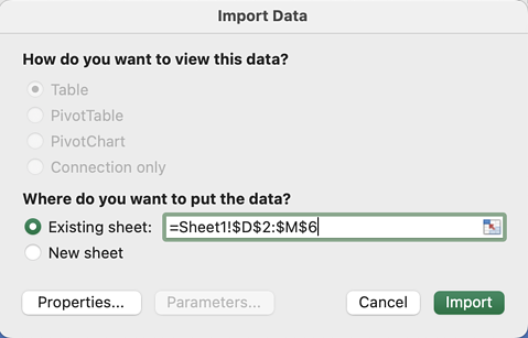
Beginning with a recent Excel file? Import your knowledge recordsdata straight into it.

Information > Get & Rework Information > Get Information. Choose the file sort to import or add through a URL and comply with the prompts to import the file into Excel.

Proceed to import all the info recordsdata into Excel.

Now, it’s good to mix the info recordsdata.

Information > Get & Rework Information > Mix Queries > Append Queries.

Choose those you need. You can too add a customized column that identifies which file the info got here from.

The VLOOKUP In Excel

The “VLOOKUP” operate works identical to VLOOKUP in Google Sheets. Right here’s an instance:

=VLOOKUP(A2, Sheet1!A:B, 2, FALSE)

This method will seek for the worth in A2 within the first column of Sheet 2 and return the corresponding worth from the second column of Sheet 2.

Use “INDEX” And “MATCH”

INDEX and MATCH work magic in Excel, too.

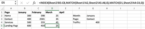
=INDEX(Sheet2!B5:C8,MATCH(Sheet1!A2,Sheet2!A5:A8,0)MATCH(D1,Sheet2!A4:C4,0))

This method works by looking out the vary on Sheet 2 (in blue) by checking the primary column (A5:A8) for no matter worth is in A2 for a precise match (0). That is all of the textual content in pink.

The inexperienced textual content is the row data. It checks the primary row (A4:C4) for no matter worth it finds in D1, on the lookout for a precise match (0).

Solely need the worth copied if the worth is a specific amount? 1 = lower than and -1 = greater than.

If that doesn’t appear all that thrilling, simply wait till you see what you are able to do with this subsequent.

Working With Information

Wanting Up Values Utilizing Two Custom-made Variables

Typically, you simply need to have the ability to lookup a selected worth.

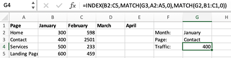
On this instance, we have now month-to-month visitors numbers within the columns and pages within the rows. Now, we are able to use INDEX and MATCH to lookup how a lot visitors the contact web page (or any web page) obtained within the month of January (or any month) simply by typing in G2 and G3.

The method you set in G4:

=INDEX(B2:C5,MATCH(G3,A2:A5,0),MATCH(G2,B1:C1,0))

INDEX must know what vary it ought to look in. Then, it needs to know which column and row it wants to seek out. The MATCH capabilities act because the row and column numbers by on the lookout for actual matches in accordance with what you typed in G2 and G3.

Which means you may transfer that little typing part to a clear sheet and arrange a dashboard so anybody in your crew can lookup knowledge!

If you happen to cherished this, strive it with SUMIFs and AVERAGEIFs, which sum (or common) knowledge based mostly on a number of standards.

That is good for shortly summarizing your Google Analytics knowledge based mostly on particular standards, akin to visitors supply, medium, and date vary.

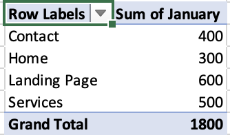
Create Pivot Tables

Pivot tables are seemingly one of the vital instruments you’ll have when attempting to summarize massive quantities of information and remodel it right into a extra manageable format.

Use it to hurry up your reporting by:

• Summarize visitors knowledge by product, class, or time interval.
• Analyze visitors over time to determine seasonal tendencies.
• Examine knowledge throughout totally different classes, akin to bounce charges for the touchdown pages for various merchandise or areas.
• Filter knowledge to indicate solely knowledge for a selected product or area.
• Calculate metrics akin to averages, counts, and percentages. For instance, the typical visitors per day for every product over the past 30 days.
• Establish outliers akin to pages or merchandise which might be promoting way more or a lot lower than different merchandise.

In Google Sheets:

Spotlight the info you need to analyze.

To make the desk: Information > Pivot Desk to open a brand new sheet with a clean pivot desk.

Now, arrange your pivot desk.

Within the “Rows” and “Columns” fields, choose the fields you need to use as rows and columns. Within the “Values” discipline, choose the sector you need to analyze.

Want one thing a little bit totally different? Customise your pivot desk by altering the abstract operate (sum, common, rely, for instance), kind and filter the info, and add subtotals and grand totals.

Professional Tip: Have a big knowledge set? Choose your complete desk by clicking on the top-left nook of the desk.

In Excel:

Identical as in sheets, begin by highlighting the info you need to analyze. For a big knowledge set, clicking on the top-left nook of the desk works right here, too.

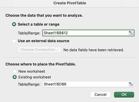
Insert > Pivot Desk > Insert the vary the place your knowledge is that you simply need to analyze. Then, if you need the pivot desk on a brand new sheet or within the present one.

(If you happen to by accident chosen an empty vary, it provides you with an error. So, if it complains, that is normally why.)

Now, arrange your pivot desk. Add no matter you need within the columns into the “Values” discipline and the rows into the “Rows” discipline.

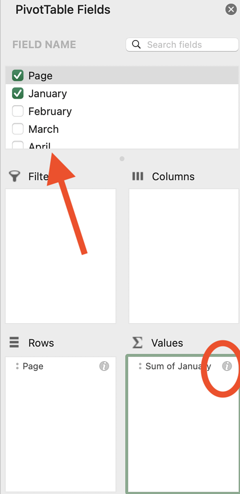
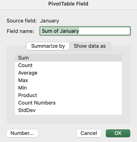
And if it’s good to change it (so it’s utilizing common as a substitute of sum, for instance), change that utilizing the data button on the suitable worth.

Use REGEXTRACT To Pull Info From URLs

The Regexextract method extracts particular knowledge from textual content strings utilizing common expressions. So, for instance, you should use Regexextract to extract the supply and medium of your web site visitors from Google Analytics studies.

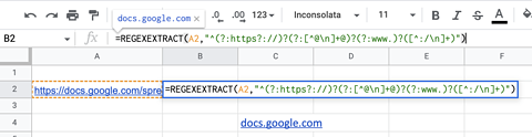
To extract the area from a URL in cell A2, you should use the next method:

=REGEXEXTRACT(A2,”^(?:https?://)?(?:[^@n]+@)?(?:www.)?([^:/n]+)”)

Common expressions might be advanced, so it’s vital to check your method with totally different examples to make sure it’s extracting the proper knowledge.

Minimizing Tables

To reduce a desk, click on on the small arrow icon within the prime left nook of the desk to break down it and conceal the info, leaving solely the desk header seen.

To broaden the desk once more, merely click on on the arrow icon.

You can too use the “Information” > “Group Rows” or “Group Columns” characteristic to group associated rows or columns collectively and create collapsible sections.

Freezing Rows And Columns

Freezing rows and columns retains particular rows or columns seen on the display screen whilst you scroll by way of the remainder of the spreadsheet.

In Google Sheets: Choose the row or column you need to freeze. Click on View > Freeze > As much as present row or column (or as much as and together with the present row/column.)

In Excel: Choose the row or column you need to freeze. Then, click on View > “Freeze Panes,” “Freeze Prime Row,” or “Freeze First Column.”

If you happen to’re actually battling a considerable amount of knowledge, strive filters. This lets you take away any irrelevant knowledge and present solely the info that meets sure standards.

Additional Ideas For Giant Information Units

Use named ranges to assign a selected identify to a variety of cells in your sheet. This could make it simpler to confer with and analyze massive knowledge units.

Keep away from utilizing too many formulation. These decelerate your sheet’s efficiency and also can make your life very tough, significantly when you begin chaining a number of formulation collectively.

Make use of conditional formatting:

In Google Sheets:

Choose the vary of cells you need to apply conditional formatting to. Click on Format > Conditional Formatting.

Within the “Conditional format guidelines” panel on the right-hand aspect of the display screen, choose the kind of formatting you need to apply. There are a number of choices to select from, together with “Coloration scale,” “Icon set,” and “Customized method is.”

In Excel:

Choose the vary of cells you need to apply conditional formatting to and click on House > Types > Conditional Formatting.

Within the drop-down menu, choose the kind of formatting you need to apply, together with “Spotlight Cells Guidelines,” “Prime/Backside Guidelines,” and “Information Bars.”

Conclusion

Excel and Google Sheets might look too simplistic to do a lot, or they may seem too sophisticated to be taught, however neither of these assumptions is true.

With a couple of formulation and methods up your sleeve, you’ll shortly discover they’re among the many strongest and vital instruments in your web optimization toolbox.

Able to grow to be an information professional? Obtain The Full Technical web optimization Audit Workbook and grasp the artwork of making ready and dealing with knowledge.

Featured Picture: Paulo Bobita/Search Engine Journal

In-post Photographs: Screenshot by writer from Excel/Google Sheets, Might 2023