
What Are Sklearn Regression Fashions?
Regression fashions are a vital part of machine studying, enabling computer systems to make predictions and perceive patterns in information with out express programming. Sklearn, a robust machine studying library, provides a spread of regression fashions to facilitate this course of.
Earlier than delving into the precise regression strategies in Sklearn, let’s briefly discover the three kinds of machine studying fashions that may be carried out utilizing Sklearn Regression Fashions:
- bolstered studying,
- unsupervised studying
- supervised studying
These fashions permit computer systems to study from information, make selections, and carry out duties autonomously. Now, let’s take a better take a look at a few of the hottest regression strategies accessible in Sklearn for implementing these fashions.
Linear Regression
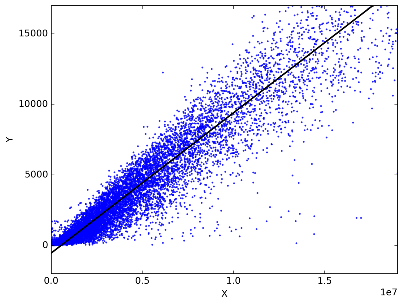
Linear regression is a statistical modeling approach that goals to determine a linear relationship between a dependent variable and a number of unbiased variables. It assumes that there’s a linear affiliation between the unbiased variables and the dependent variable, and that the residuals (the variations between the precise and predicted values) are usually distributed.
Working precept of linear regression
The working precept of linear regression includes becoming a line to the info factors that minimizes the sum of squared residuals. This line represents the perfect linear approximation of the connection between the unbiased and dependent variables. The coefficients (slope and intercept) of the road are estimated utilizing the least squares technique.
Implementation of linear regression utilizing sklearn
Sklearn supplies a handy implementation of linear regression by way of its LinearRegression class. Here is an instance of use it:
from sklearn.linear_model import LinearRegression
# Create an occasion of the LinearRegression mannequin
mannequin = LinearRegression()
# Match the mannequin to the coaching information
mannequin.match(X_train, y_train)
# Predict the goal variable for brand new information
y_pred = mannequin.predict(X_test)
Polynomial Regression
Polynomial regression is an extension of linear regression that permits for capturing nonlinear relationships between variables by including polynomial phrases. It includes becoming a polynomial operate to the info factors, enabling extra versatile modeling of complicated relationships between the unbiased and dependent variables.
Benefits and limitations of polynomial regression
The important thing benefit of polynomial regression is its potential to seize nonlinear patterns within the information, offering a greater match than linear regression in such circumstances. Nevertheless, it may be liable to overfitting, particularly with high-degree polynomials. Moreover, decoding the coefficients of polynomial regression fashions could be difficult.
Making use of polynomial regression with sklearn
Sklearn makes it easy to implement polynomial regression. Here is an instance:
from sklearn.preprocessing import PolynomialFeatures
from sklearn.linear_model import LinearRegression
from sklearn.pipeline import make_pipeline
# Create polynomial options
poly_features = PolynomialFeatures(diploma=2)
X_poly = poly_features.fit_transform(X)
# Create a pipeline with polynomial regression
mannequin = make_pipeline(poly_features, LinearRegression())
# Match the mannequin to the coaching information
mannequin.match(X_train, y_train)
# Predict the goal variable for brand new information
y_pred = mannequin.predict(X_test)
Within the code snippet above, X represents the unbiased variable values, X_poly incorporates the polynomial options created utilizing PolynomialFeatures, and y represents the corresponding goal variable values. The pipeline combines the polynomial options and the linear regression mannequin for seamless implementation.
Evaluating polynomial regression fashions
Analysis of polynomial regression fashions could be achieved utilizing comparable metrics as in linear regression, corresponding to MSE, R rating, and RMSE. Moreover, visible inspection of the mannequin’s match to the info and residual evaluation can present insights into its efficiency.
Polynomial regression is a robust software for capturing complicated relationships, but it surely requires cautious tuning to keep away from overfitting. By leveraging Sklearn’s performance, implementing polynomial regression fashions and evaluating their efficiency turns into extra accessible and environment friendly.
Ridge Regression
Ridge regression is a regularized linear regression approach that introduces a penalty time period to the loss operate, aiming to scale back the affect of multicollinearity amongst unbiased variables. It shrinks the regression coefficients, offering extra secure and dependable estimates.
The motivation behind ridge regression is to mitigate the problems brought on by multicollinearity, the place unbiased variables are extremely correlated. By including a penalty time period, ridge regression helps forestall overfitting and improves the mannequin’s generalization potential.
Implementing ridge regression utilizing sklearn
Sklearn supplies a easy solution to implement ridge regression. Here is an instance:
from sklearn.linear_model import Ridge
# Create an occasion of the Ridge regression mannequin
mannequin = Ridge(alpha=0.5)
# Match the mannequin to the coaching information
mannequin.match(X_train, y_train)
# Predict the goal variable for brand new information
y_pred = mannequin.predict(X_test)
Within the code snippet above, X_train represents the coaching information with unbiased variables, y_train represents the corresponding goal variable values, and X_test is the brand new information for which we wish to predict the goal variable (y_pred). The alpha parameter controls the power of the regularization.
To evaluate the efficiency of ridge regression fashions, comparable analysis metrics as in linear regression can be utilized, corresponding to MSE, R rating, and RMSE. Moreover, cross-validation and visualization of the coefficients’ magnitude can present insights into the mannequin’s efficiency and the affect of regularization.
Lasso Regression
Lasso regression is a linear regression approach that includes L1 regularization, selling sparsity within the mannequin by shrinking coefficients in the direction of zero. It may be helpful for characteristic choice and dealing with multicollinearity.
Lasso regression can successfully deal with datasets with a lot of options and routinely choose related variables. Nevertheless, it tends to pick out just one variable from a gaggle of extremely correlated options, which generally is a limitation.
Using lasso regression in sklearn
Sklearn supplies a handy implementation of lasso regression. Here is an instance:
from sklearn.linear_model import Lasso
# Create an occasion of the Lasso regression mannequin
mannequin = Lasso(alpha=0.5)
# Match the mannequin to the coaching information
mannequin.match(X_train, y_train)
# Predict the goal variable for brand new information
y_pred = mannequin.predict(X_test)
Within the code snippet above, X_train represents the coaching information with unbiased variables, y_train represents the corresponding goal variable values, and X_test is the brand new information for which we wish to predict the goal variable (y_pred). The alpha parameter controls the power of the regularization.
Evaluating lasso regression fashions
Analysis of lasso regression fashions could be achieved utilizing comparable metrics as in linear regression, corresponding to MSE, R rating, and RMSE. Moreover, analyzing the coefficients’ magnitude and sparsity sample can present insights into characteristic choice and the affect of regularization.
Help Vector Regression (SVR)
Help Vector Regression (SVR) is a regression approach that makes use of the rules of Help Vector Machines. It goals to discover a hyperplane that most closely fits the info whereas permitting a tolerance margin for errors.
SVR employs kernel features to rework the enter variables into higher-dimensional characteristic house, enabling the modeling of complicated relationships. Well-liked kernel features embrace linear, polynomial, radial foundation operate (RBF), and sigmoid.
Implementing SVR with sklearn
Sklearn provides an implementation of SVR. Here is an instance:
from sklearn.svm import SVR
# Create an occasion of the SVR mannequin
mannequin = SVR(kernel="rbf", C=1.0, epsilon=0.1)
# Match the mannequin to the coaching information
mannequin.match(X_train, y_train)
# Predict the goal variable for brand new information
y_pred = mannequin.predict(X_test)
Within the code snippet above, X_train represents the coaching information with unbiased variables, y_train represents the corresponding goal variable values, and X_test is the brand new information for which we wish to predict the goal variable (y_pred). The kernel parameter specifies the kernel operate, C controls the regularization, and epsilon units the tolerance for errors.
Evaluating SVR fashions
SVR fashions could be evaluated utilizing customary regression metrics like MSE, R rating, and RMSE. It is also useful to investigate the residuals and visually examine the mannequin’s match to the info for assessing its efficiency and capturing any patterns or anomalies.
Determination Tree Regression
Determination tree regression is a non-parametric supervised studying algorithm that builds a tree-like mannequin to make predictions. It partitions the characteristic house into segments and assigns a relentless worth to every area. For a extra detailed introduction and examples, you’ll be able to click on right here: resolution tree introduction.

Making use of resolution tree regression utilizing sklearn
Sklearn supplies an implementation of resolution tree regression by way of the DecisionTreeRegressor class. It permits customization of parameters corresponding to most tree depth, minimal pattern cut up, and the selection of splitting criterion.
Analysis of resolution tree regression fashions includes utilizing metrics like MSE, R rating, and RMSE. Moreover, visualizing the choice tree construction and analyzing characteristic significance can present insights into the mannequin’s conduct.
Random Forest Regression
Random forest regression is an ensemble studying technique that mixes a number of resolution bushes to make predictions. It reduces overfitting and improves prediction accuracy by aggregating the predictions of particular person bushes.
Random forest regression provides robustness, handles high-dimensional information, and supplies characteristic significance evaluation. Nevertheless, it may be computationally costly and fewer interpretable in comparison with single resolution bushes.
Implementing random forest regression with sklearn
Sklearn supplies a simple solution to implement random forest regression. Here is an instance:
from sklearn.ensemble import RandomForestRegressor
# Create an occasion of the Random Forest regression mannequin
mannequin = RandomForestRegressor(n_estimators=100)
# Match the mannequin to the coaching information
mannequin.match(X_train, y_train)
# Predict the goal variable for brand new information
y_pred = mannequin.predict(X_test)
Within the code snippet above, X_train represents the coaching information with unbiased variables, y_train represents the corresponding goal variable values, and X_test is the brand new information for which we wish to predict the goal variable (y_pred). The n_estimators parameter specifies the variety of bushes within the random forest.
Evaluating random forest regression fashions
Analysis of random forest regression fashions includes utilizing metrics like MSE, R rating, and RMSE. Moreover, analyzing characteristic significance and evaluating with different regression fashions can present insights into the mannequin’s efficiency and robustness.
Gradient Boosting Regression
Gradient boosting regression is an ensemble studying approach that mixes a number of weak prediction fashions, usually resolution bushes, to create a powerful predictive mannequin. It iteratively improves predictions by minimizing the errors of earlier iterations.
Gradient boosting regression provides excessive predictive accuracy, handles several types of information, and captures complicated interactions. Nevertheless, it may be computationally intensive and liable to overfitting if not correctly tuned.

Using gradient boosting regression in sklearn
Sklearn supplies an implementation of gradient boosting regression by way of the GradientBoostingRegressor class. It permits customization of parameters such because the variety of boosting levels, studying fee, and most tree depth.
Evaluating gradient boosting regression fashions
Analysis of gradient boosting regression fashions includes utilizing metrics like MSE, R rating, and RMSE. Moreover, analyzing characteristic significance and tuning hyperparameters can optimize mannequin efficiency. For a extra detailed introduction and examples, you’ll be able to click on right here: gradient boosting resolution bushes in Python.
Conclusion
In conclusion, we explored varied regression fashions and mentioned the significance of selecting the suitable mannequin for correct predictions. Sklearn’s regression fashions provide a robust and versatile toolkit for predictive evaluation, enabling information scientists to make knowledgeable selections primarily based on information.
The publish Mastering Regression Evaluation with Sklearn: Unleashing the Energy of Sklearn Regression Fashions appeared first on Datafloq.