
As information lovers, we love uncovering tales in datasets. With Posit’s RStudio Desktop and Databricks, you’ll be able to analyze information with dplyr, create spectacular graphs with ggplot2 and weave information narratives with Quarto, all utilizing information that’s saved in Databricks.
Posit and Databricks not too long ago introduced a strategic partnership to offer a simplified expertise for Posit and Databricks customers. By combining Posit’s RStudio with Databricks, you’ll be able to dive into any information saved on the Databricks Lakehouse Platform, from small information units to massive streaming information. Posit offers information scientists with user-friendly and code-first environments and instruments for working with information and writing code. Databricks offers a scaleable end-to-end structure for information storage, compute, AI and governance.
One goal for the partnership is to enhance help for Spark Join in R via sparklyr, simplifying the method of connecting to Databricks clusters through Databricks Join. Sooner or later, Posit and Databricks will provide streamlined integration to automate many of those steps.
At the moment, we’ll take a tour of the improved sparklyr expertise with the New York Metropolis taxi journey document information that has over 10,000,000 rows and a complete file measurement of 37 gigabytes.
Arrange your surroundings
To start, it’s essential to arrange the connection between RStudio and Databricks.
Save your surroundings variables
To make use of Databricks Join, you want three configuration objects. Log in to a Databricks account to acquire:
- The Workspace Occasion URL, which seems to be like
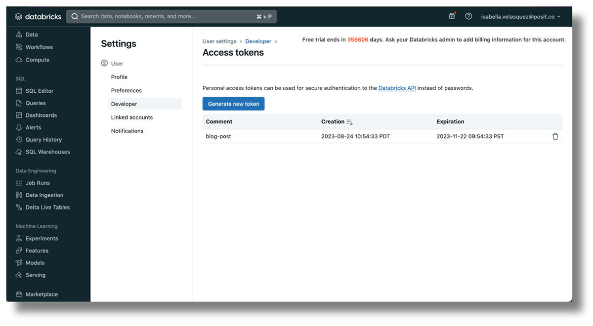
https://databricks-instance.cloud.databricks.com/?o=12345678910111213 - An entry token to authenticate the account. Click on the person title on the top-right nook, choose “Consumer Settings”, then “Developer”. Click on “Handle” subsequent to “Entry Tokens” after which “Generate new token”. Copy the token, because it will not be proven once more.
- The Cluster ID of a presently operating cluster throughout the workspace. Set one up by navigating to
https://<databricks-instance>/#/setting/clusters/. Extra data might be discovered within the Databricks docs. Alternatively, go to “Compute” within the sidebar and add a cluster.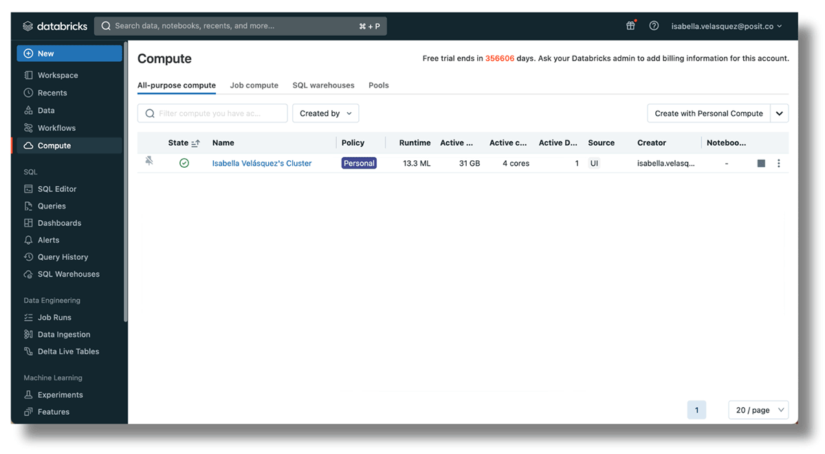
Now, head to RStudio.
To securely join your Databricks and RStudio accounts, set the Databricks Workspace, entry token and cluster ID as surroundings variables. Setting variables hold delicate data outdoors of your code, decreasing the chance of exposing confidential information in your scripts.
The usethis package deal has a useful perform for opening the R surroundings. Run the code beneath in your console to entry the .Renviron file:
usethis::edit_r_environ()This perform mechanically opens the .Renviron file for enhancing. Arrange the Databricks Workspace URL, entry token and cluster ID within the .Renviron file with the next names: DATABRICKS_HOST for the URL, DATABRICKS_TOKEN for the entry token and DATABRICKS_CLUSTER_ID for the cluster ID. For instance:
DATABRICKS_HOST=https://databricks-instance.cloud.databricks.com/?o=12345678910111213
DATABRICKS_TOKEN=1ab2cd3ef45ghijklmn6o78qrstuvwxyz
DATABRICKS_CLUSTER_ID=1234-567891-1a23bcde
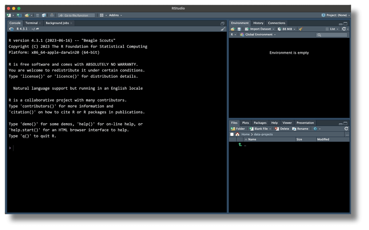
Your RStudio could seem like this:

Save the .Renviron file and restart the R session. Now, your surroundings is ready up to hook up with Databricks!
Set up required packages
The sparklyr package deal is a robust R package deal that lets you work with Apache Spark, a collection of knowledge processing, SQL and superior analytics APIs. With sparklyr, you’ll be able to leverage the capabilities of Spark immediately from throughout the R surroundings. Connections made with sparklyr can even leverage the Connections Pane, a user-friendly approach to navigate and think about your information.
Posit has been working to replace and enhance the sparklyr package deal. Spark Join requires a device known as gRPC to work. The Spark crew presents two methods to make use of it: one with Scala and the opposite with Python. Within the growth model of sparklyr, we use reticulate so as to add options like dplyr, DBI help and integration with RStudio’s Connection pane to the Python API. To make enhancements and fixes quicker, we have separated the Python half into its personal package deal, pysparklyr.
Entry the brand new capabilities of sparklyr by putting in the event variations of sparklyr and pysparklyr in RStudio:
library(remotes)
install_github("sparklyr/sparklyr")
install_github("mlverse/pysparklyr")
The sparklyr package deal requires particular Python elements to speak with Databricks Join. To arrange these elements, run the next helper perform:
pysparklyr::install_pyspark()Now, you’ll be able to load the sparklyr package deal. Sparklyr will choose up on the preset surroundings variables that you just configured above.
library(sparklyr)Subsequent, use spark_connect() to open the connection to Databricks. You possibly can inform sparklyr that you’re connecting to a Spark cluster by setting methodology = "databricks_connect".
sc <- spark_connect(methodology = "databricks_connect")If the next error pops up:
# Error in `import_check()`:
# ! Python library 'databricks.join' will not be out there within the
#   'r-sparklyr' digital surroundings. Set up all the wanted python libraries
#   utilizing: pysparklyr::install_pyspark(virtualenv_name = "r-sparklyr")
Run the supplied script to put in the required Python packages:
pysparklyr::install_pyspark(virtualenv_name = "r-sparklyr")With that, you need to see the information within the Connections pane within the higher right-hand of RStudio.

Congratulations, you have linked your session with Databricks!
Retrieve and analyze your information
RStudio can connect with many databases directly. Utilizing the RStudio Connections Pane, you’ll be able to verify which databases you are linked to and see which of them are presently in use.

The brand new integration with Spark lets you browse information managed in Unity Catalog, populating the Connections Pane with the identical construction discovered within the Databricks Information Explorer.
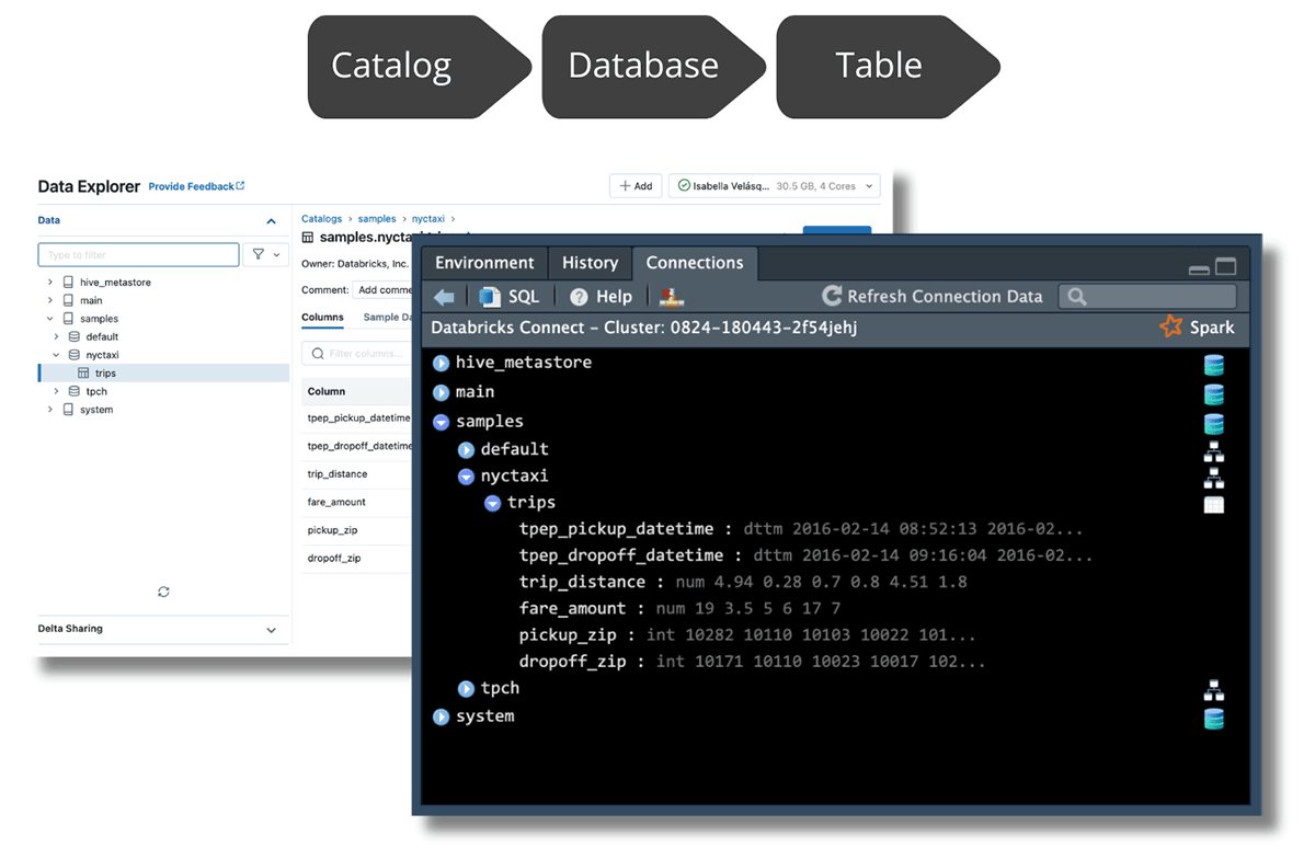
In RStudio, you’ll be able to navigate the information by increasing from the highest degree all the best way all the way down to the desk you want to discover. If you develop the desk, you’ll be able to see its columns and information varieties. You may as well click on on the desk icon on the proper facet of the desk title, to see the primary 1,000 rows of the information:

Entry information utilizing the Databricks connection
The dbplyr package deal bridges R and databases by permitting you to entry distant database tables as in the event that they had been in-memory information frames. As well as, it interprets dplyr verbs into SQL queries, making it straightforward to work with the database information utilizing acquainted R syntax.
As soon as your connection to Databricks has been arrange, you should use dbplyr’s tbl() and in_catalog() capabilities to entry any desk following the order of ranges within the catalog: Catalog, Database and Desk.
Within the instance beneath, "samples" is the Catalog, "nytaxi" is the Database and "journeys" is the Desk. Save the desk reference within the object journeys.
library(dplyr)
library(dbplyr)

journeys <- tbl(sc, in_catalog("samples", "nyctaxi", "journeys"))

journeys

# Supply: spark<samples.nyctaxi.journeys> [?? x 6]
   tpep_pickup_datetime tpep_dropoff_datetime trip_distance fare_amount
   <dttm>               <dttm>                        <dbl>       <dbl>
 1 2016-02-14 08:52:13  2016-02-14 09:16:04            4.94        19
 2 2016-02-04 10:44:19  2016-02-04 10:46:00            0.28         3.5
 3 2016-02-17 09:13:57  2016-02-17 09:17:55            0.7          5
 4 2016-02-18 02:36:07  2016-02-18 02:41:45            0.8          6
 5 2016-02-22 06:14:41  2016-02-22 06:31:52            4.51        17
 6 2016-02-04 22:45:02  2016-02-04 22:50:26            1.8          7
 7 2016-02-15 07:03:28  2016-02-15 07:18:45            2.58        12
 8 2016-02-25 11:09:26  2016-02-25 11:24:50            1.4         11
 9 2016-02-13 08:28:18  2016-02-13 08:36:36            1.21         7.5
10 2016-02-13 16:03:48  2016-02-13 16:10:24            0.6          6
# ℹ extra rows
# ℹ 2 extra variables: pickup_zip <int>, dropoff_zip <int>
Now, you’ll be able to proceed to work with the journeys information!
Question the information and get outcomes again
Since you may have accessed the information through dplyr, you’ll be able to carry out information manipulations utilizing your favourite dplyr capabilities. Beneath, we use the brand new native R pipe |> launched in R 4.1. You may additionally use the magrittr pipe %>% to your dplyr operations. To study extra about this native R pipe and the way it differs from the magrittr pipe, go to the tidyverse weblog.
You possibly can clear and discover the dataset by utilizing dplyr instructions on the taxi object. In keeping with the NYC Taxi & Limousine Fee, the preliminary cab fare for taxis is $3. To take away information factors beneath $3, you should use filter(). If you wish to discover out extra about cab fares, you should use summarize() to calculate the minimal, common, and most fare quantities.
journeys |>
  filter(fare_amount > 3) |>
  summarize(
    min_fare = min(fare_amount, na.rm = TRUE),
    avg_fare = imply(fare_amount, na.rm = TRUE),
    max_fare = max(fare_amount, na.rm = TRUE)
  )

# Supply: spark<?> [?? x 3]
  min_fare avg_fare max_fare
     <dbl>    <dbl>    <dbl>
1      3.5     12.4      275
The minimal fare quantity is $3.50, the common fare quantity for a cab journey was $12.40, and the utmost fare was $275!
You possibly can visualize your information to get a way of the distribution of the fare quantities:
library(ggplot2)

journeys |>
  ggplot(aes(x = fare_amount)) +
  geom_density() +
  theme_minimal() +
  labs(title = "Density Plot of NYC Taxi Fare Quantities",
       xlab = "Fare Quantity",
       ylab = "Density")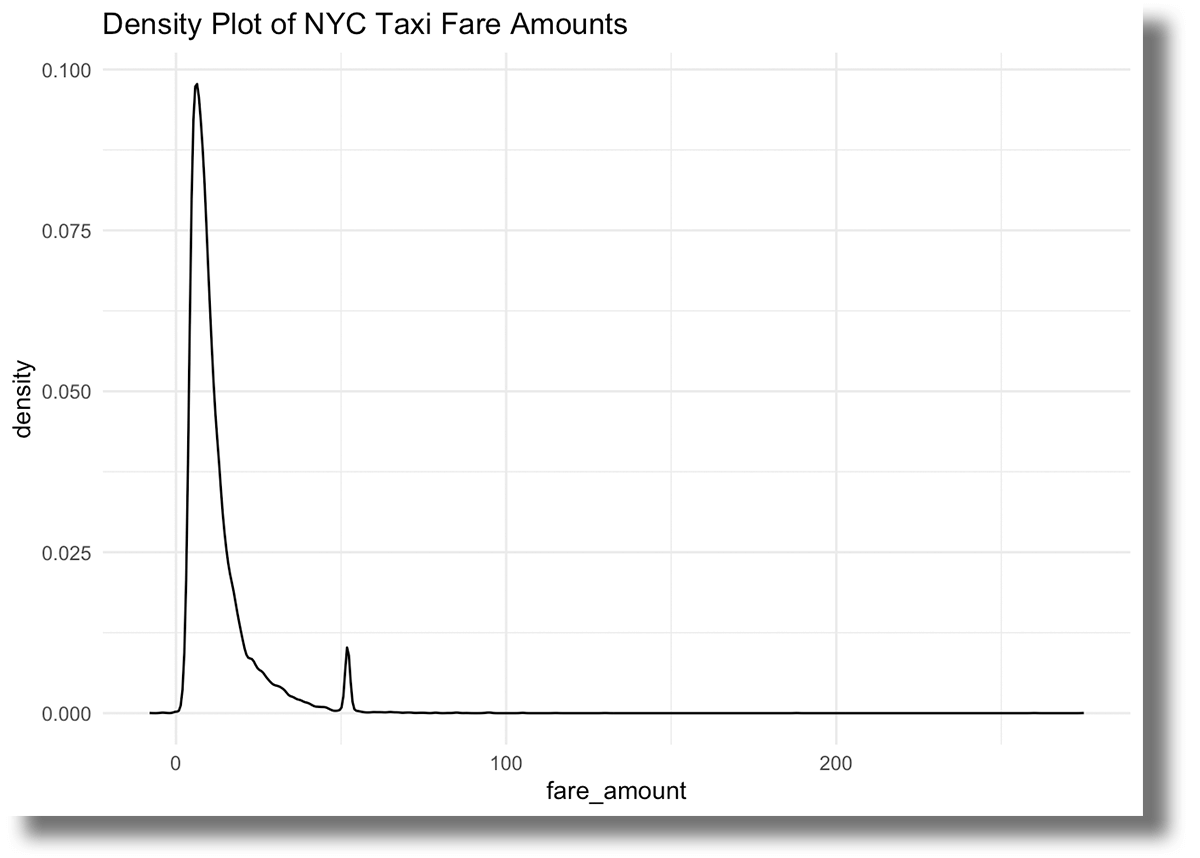
Whereas most journeys are decrease than $25, you’ll be able to see a excessive variety of fares totaling simply over $50. This may be because of mounted charges for rides from the airports to town.
Now that you’ve a way of the distribution of fare quantities, let’s create one other visualization. Within the following instance, you create a brand new column known as hour to point out the time of day for every taxi journey. Then, you should use ggplot2 to create a {custom} visualization that shows how the fares are distributed at totally different occasions of the day.
journeys |>
  filter(fare_amount > 3) |>
  mutate(
    hour = case_when(
      lubridate::hour(tpep_pickup_datetime) >= 18 ~ "Night",
      lubridate::hour(tpep_pickup_datetime) >= 12 &
        lubridate::hour(tpep_pickup_datetime) < 18 ~ "Afternoon",
      lubridate::hour(tpep_pickup_datetime) >= 6 &
        lubridate::hour(tpep_pickup_datetime) < 12 ~ "Morning",
      lubridate::hour(tpep_pickup_datetime) < 6 ~ "Night time"
    )
  ) |>

  ggplot(aes(x = hour, y = fare_amount)) +
  ggdist::stat_halfeye(
    regulate = .5,
    width = .6,
    .width = 0,
    justification = -.3,
    point_colour = NA,
    aes(fill = hour)
  ) +
  geom_point(
    measurement = 1.5,
    alpha = .3,
    place = position_jitter(seed = 1, width = .1),
    aes(colour = hour)
  ) +
  coord_flip() +
  theme_minimal() +
  labs(title = "Distribution of NYC Taxi Fare Quantities by Time of Day",
       y = "Fare Quantity ($)",
       x = "Time of Day") +
  theme(legend.place = "none") +
  scale_color_manual(
    values = c(
      "Morning" = "#70A3A6",
      "Afternoon" = "#8AA67A",
      "Night" = "#BF96A3",
      "Night time" = "#E58066"
    )
  ) +
  scale_fill_manual(
    values = c(
      "Morning" = "#1F4F4F",
      "Afternoon" = "#3B4F29",
      "Night" = "#542938",
      "Night time" = "#80361C"
    )
  )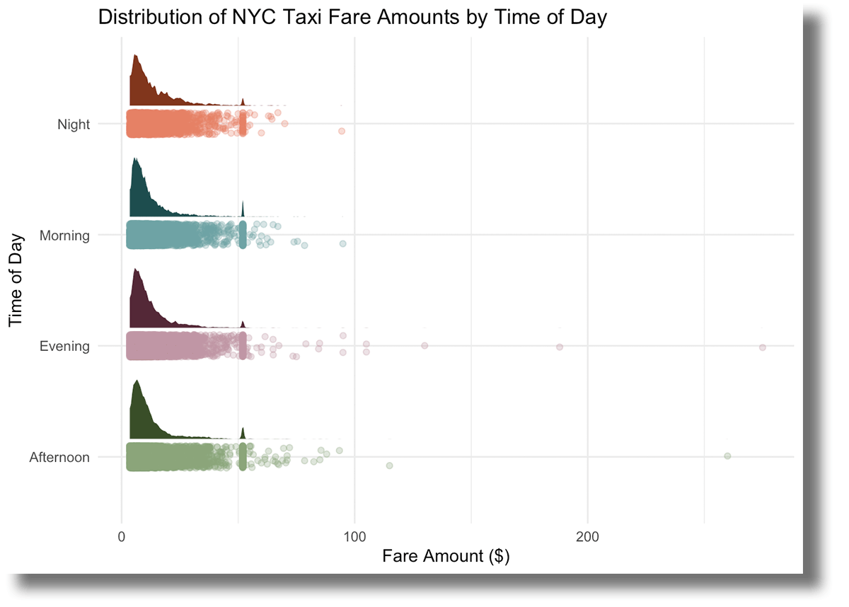
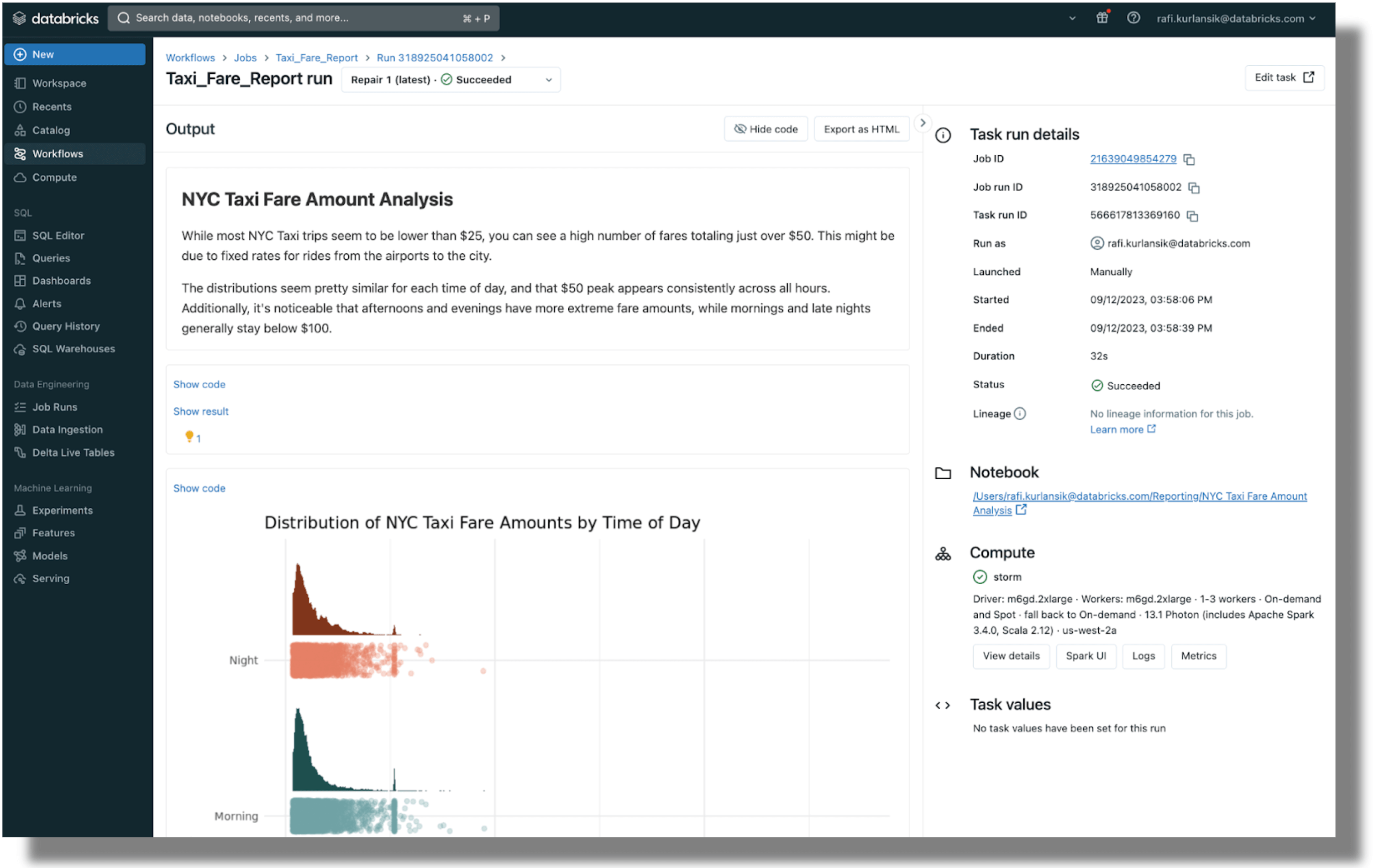
The distributions appear fairly comparable for every time of day, and that $50 peak seems constantly throughout all hours. Moreover, it is noticeable that afternoons and evenings have extra excessive fare quantities, whereas mornings and late nights typically keep beneath $100.
Nice, you have dug into your dataset. Now, it is time to create one thing to publish!
Publish your content material and share your insights
Why uncover fantastic tales if you cannot share them with the world? This brings us to the ultimate chapter of the journey – publishing your content material.
The upgrades to sparklyr permit you to create complete, visually interesting reviews in RStudio utilizing the processing energy of Databricks. Upon getting queried your information and investigated the story you wish to inform, you’ll be able to proceed to create a report utilizing Quarto:
---
title: "NYC Taxi Fare Quantity Evaluation"
---
Whereas most NYC Taxi journeys appear to be decrease than $25, you'll be able to see a excessive quantity of fares totaling simply over $50. This may be due to mounted charges for rides from the airports to town.

The distributions appear fairly comparable for every time of day, and that $50 peak seems constantly throughout all hours. Moreover, it's noticeable that afternoons and evenings have extra excessive fare quantities, whereas mornings and late nights typically keep beneath $100.

```{r}
#| echo: false
supply(right here::right here("1_user-story-reporting",
                  "plot_script.R"))
```

::: {structure="[[1, 1], [1]]"}

```{r}
density_plot
```

```{r}
corr_plot
```

```{r}
wday_plot
```
:::
Rendering the .qmd file, you generate a visually interesting report because the output:

To publish this report, you may have a number of choices. Posit presents Posit Join, an enterprise-level platform for deploying R and Python information merchandise. Information scientists use Posit Hook up with automate time-consuming duties with code, distribute custom-built instruments and options throughout groups, and securely share insights with decision-makers.

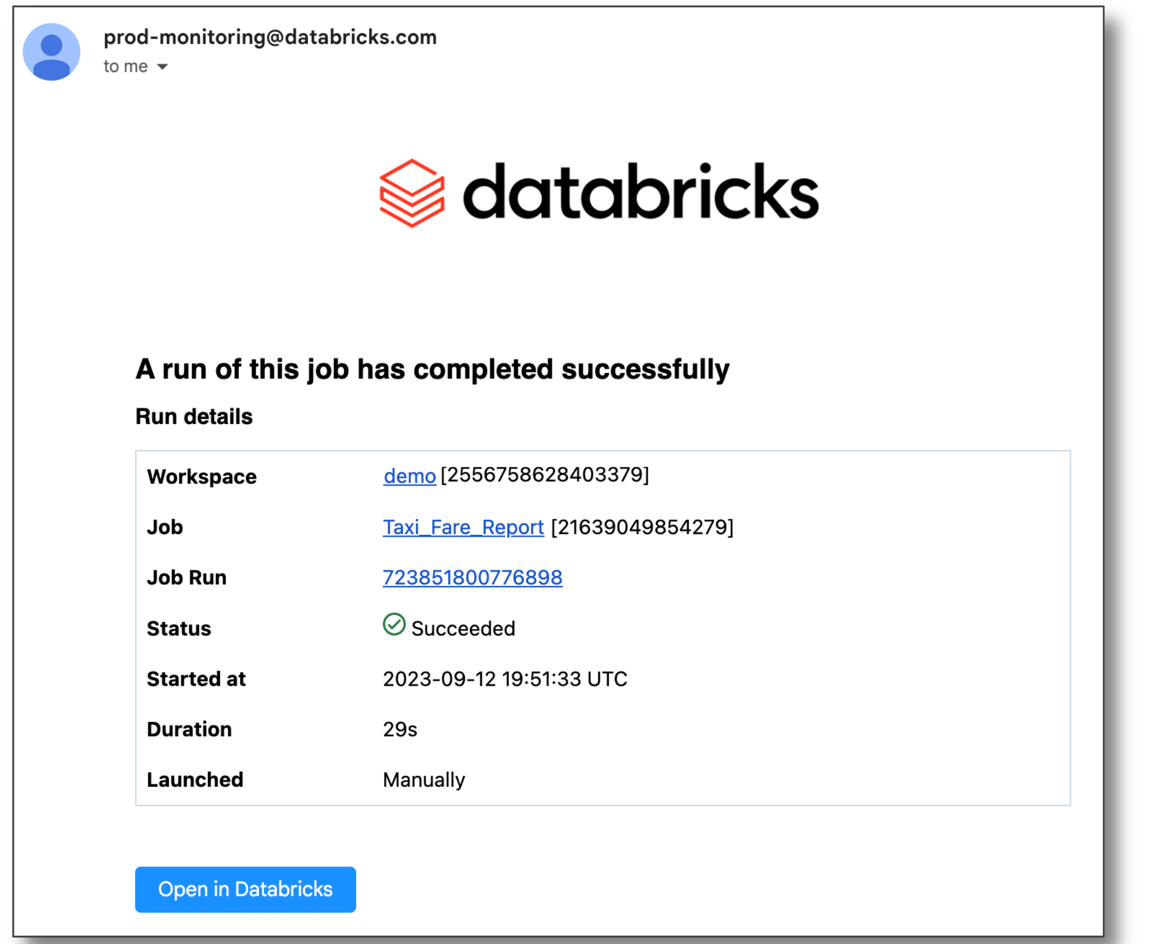
To publish the report via Databricks, you’ll be able to schedule it as a pocket book job and electronic mail a hyperlink to the output to stakeholders.
You may as well publish Quarto paperwork on Quarto Pub and GitHub Pages. Discover out extra on Quarto’s publishing information.
Disconnect from the server
As soon as you’re finished along with your evaluation, you wish to be sure you disconnect from Spark Join.
spark_disconnect(sc)Attempt RStudio with Databricks
The mixing between RStudio and Databricks permits customers to get the advantages of each, whereas getting a simplified developer expertise. Attempt it out your self with this documentation.