Construct an Amazon Redshift information warehouse utilizing an Amazon DynamoDB single-table design

Amazon DynamoDB is a completely managed NoSQL service that delivers single-digit millisecond efficiency at any scale. It’s utilized by 1000’s of consumers for mission-critical workloads. Typical use instances for DynamoDB are an ecommerce utility dealing with a excessive quantity of transactions, or a gaming utility that should keep scorecards for gamers and video games. In conventional databases, we might mannequin such functions utilizing a normalized information mannequin (entity-relation diagram). This method comes with a heavy computational price when it comes to processing and distributing the information throughout a number of tables whereas making certain the system is ACID-compliant always, which might negatively affect efficiency and scalability. If these entities are incessantly queried collectively, it is sensible to retailer them in a single desk in DynamoDB. That is the idea of single-table design. Storing various kinds of information in a single desk means that you can retrieve a number of, heterogeneous merchandise sorts utilizing a single request. Such requests are comparatively simple, and often take the next type:

SELECT * FROM TABLE WHERE Some_Attribute="some_value"

On this format, some_attribute is a partition key or a part of an index.

Nonetheless, most of the identical prospects utilizing DynamoDB would additionally like to have the ability to carry out aggregations and advert hoc queries in opposition to their information to measure vital KPIs which are pertinent to their enterprise. Suppose we’ve a profitable ecommerce utility dealing with a excessive quantity of gross sales transactions in DynamoDB. A typical ask for this information could also be to determine gross sales developments in addition to gross sales development on a yearly, month-to-month, and even day by day foundation. A lot of these queries require complicated aggregations over a lot of information. A key pillar of AWS’s fashionable information technique is using purpose-built information shops for particular use instances to attain efficiency, price, and scale. Deriving enterprise insights by figuring out year-on-year gross sales development is an instance of a web based analytical processing (OLAP) question. A lot of these queries are suited to an information warehouse.

The purpose of an information warehouse is to allow companies to investigate their information quick; that is vital as a result of it means they’re able to achieve beneficial insights in a well timed method. Amazon Redshift is totally managed, scalable, cloud information warehouse. Constructing a performant information warehouse is non-trivial as a result of the information must be extremely curated to function a dependable and correct model of the reality.

On this submit, we stroll by the method of exporting information from a DynamoDB desk to Amazon Redshift. We talk about information mannequin design for each NoSQL databases and SQL information warehouses. We start with a single-table design as an preliminary state and construct a scalable batch extract, load, and remodel (ELT) pipeline to restructure the information right into a dimensional mannequin for OLAP workloads.

DynamoDB desk instance

We use an instance of a profitable ecommerce retailer permitting registered customers to order merchandise from their web site. A easy ERD (entity-relation diagram) for this utility could have 4 distinct entities: prospects, addresses, orders, and merchandise. For purchasers, we’ve data reminiscent of their distinctive person identify and e mail deal with; for the deal with entity, we’ve a number of buyer addresses. Orders comprise data relating to the order positioned, and the merchandise entity supplies details about the merchandise positioned in an order. As we are able to see from the next diagram, a buyer can place a number of orders, and an order should comprise a number of merchandise.

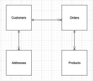
We might retailer every entity in a separate desk in DynamoDB. Nonetheless, there isn’t a strategy to retrieve buyer particulars alongside all of the orders positioned by the client with out making a number of requests to the client and order tables. That is inefficient from each a value and efficiency perspective. A key purpose for any environment friendly utility is to retrieve all of the required data in a single question request. This ensures quick, constant efficiency. So how can we rework our information to keep away from making a number of requests? One choice is to make use of single-table design. Benefiting from the schema-less nature of DynamoDB, we are able to retailer various kinds of information in a single desk in an effort to deal with totally different entry patterns in a single request. We will go additional nonetheless and retailer various kinds of values in the identical attribute and use it as a world secondary index (GSI). That is known as index overloading.

A typical entry sample we could need to deal with in our single desk design is to get buyer particulars and all orders positioned by the client.

To accommodate this entry sample, our single-table design appears like the next instance.

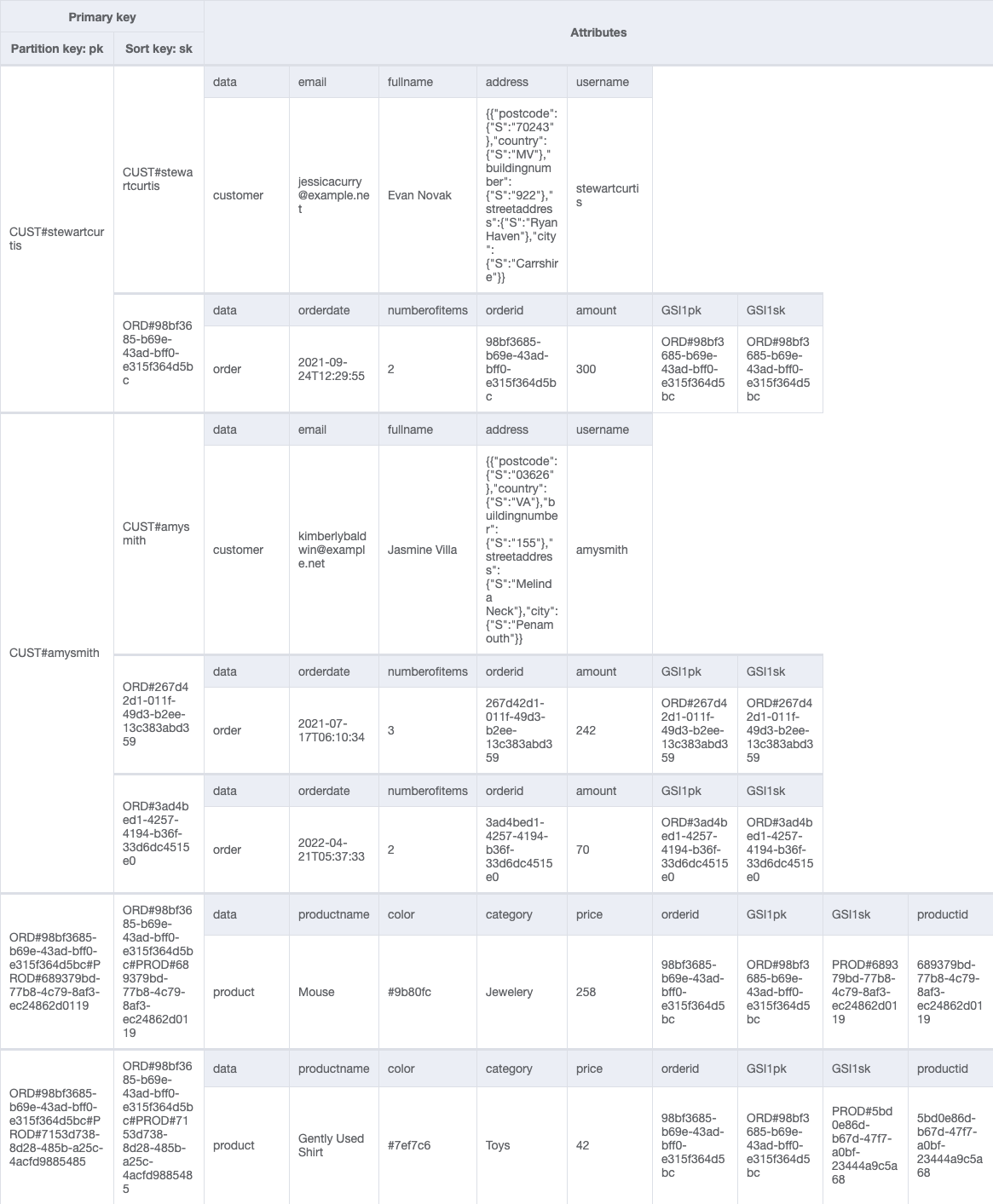
By proscribing the variety of addresses related to a buyer, we are able to retailer deal with particulars as a posh attribute (moderately than a separate merchandise) with out exceeding the 400 KB merchandise measurement restrict of DynamoDB.

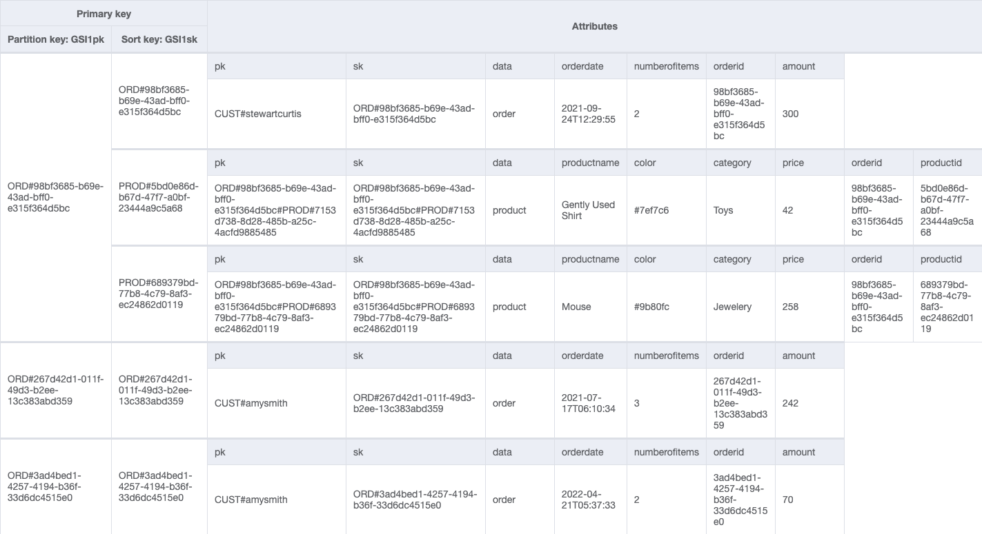
We will add a world secondary index (GSIpk and GSIsk) to seize one other entry sample: get order particulars and all product gadgets positioned in an order. We use the next desk.

We’ve used generic attribute names, PK and SK, for our partition key and type key columns. It’s because they maintain information from totally different entities. Moreover, the values in these columns are prefixed by generic phrases reminiscent of CUST# and ORD# to assist us determine the kind of information we’ve and be certain that the worth in PK is exclusive throughout all information within the desk.

A well-designed single desk is not going to solely cut back the variety of requests for an entry sample, however will service many various entry patterns. The problem comes when we have to ask extra complicated questions of our information, for instance, what was the year-on-year quarterly gross sales development by product damaged down by nation?

The case for an information warehouse

A knowledge warehouse is ideally suited to reply OLAP queries. Constructed on extremely curated structured information, it supplies the flexibleness and pace to run aggregations throughout a complete dataset to derive insights.

To deal with our information, we have to outline an information mannequin. An optimum design selection is to make use of a dimensional mannequin. A dimension mannequin consists of truth tables and dimension tables. Truth tables retailer the numeric details about enterprise measures and overseas keys to the dimension tables. Dimension tables retailer descriptive details about the enterprise details to assist perceive and analyze the information higher. From a enterprise perspective, a dimension mannequin with its use of details and dimensions can current complicated enterprise processes in a simple-to-understand method.

Constructing a dimensional mannequin

A dimensional mannequin optimizes learn efficiency by environment friendly joins and filters. Amazon Redshift robotically chooses the perfect distribution type and type key primarily based on workload patterns. We construct a dimensional mannequin from the one DynamoDB desk primarily based on the next star schema.

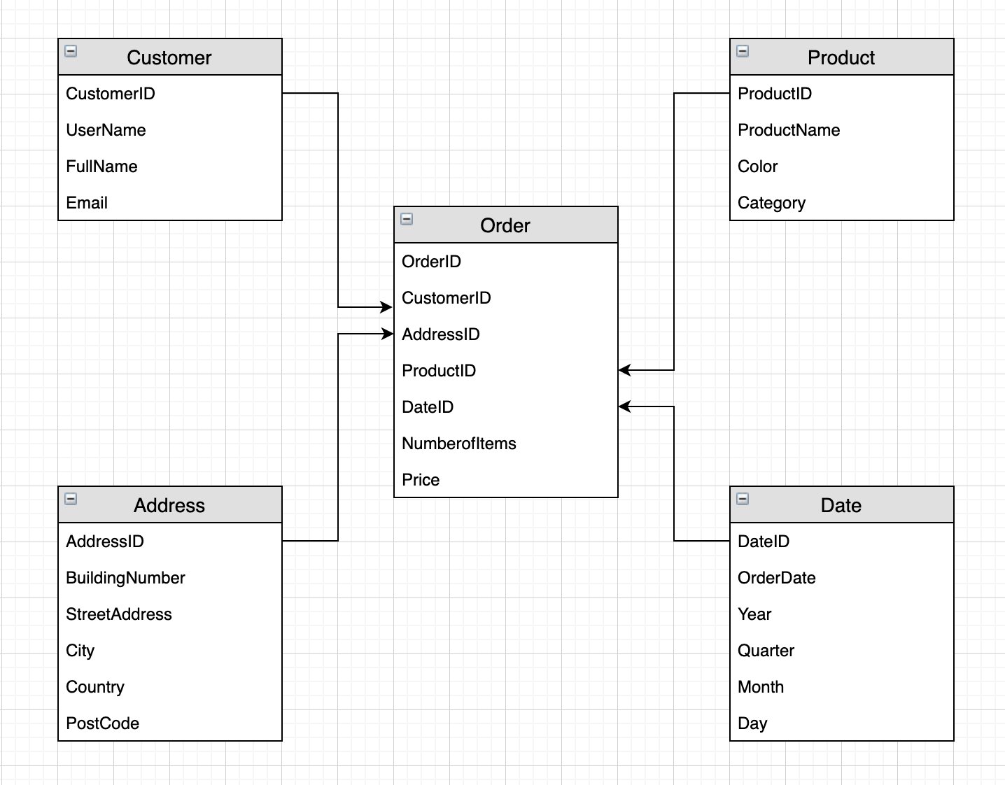
We’ve separated every merchandise kind into particular person tables. We’ve a single truth desk (Orders) containing the enterprise measures worth and numberofitems, and overseas keys to the dimension tables. By storing the worth of every product within the truth desk, we are able to monitor worth fluctuations within the truth desk with out regularly updating the product dimension. (In an identical vein, the DynamoDB attribute quantity is an easy derived measure in our star schema: quantity is the summation of product costs per orderid).

By splitting the descriptive content material of our single DynamoDB desk into a number of Amazon Redshift dimension tables, we are able to take away redundancy by solely holding in every dimension the data pertinent to it. This enables us the flexibleness to question the information beneath totally different contexts; for instance, we could need to know the frequency of buyer orders by metropolis or product gross sales by date. The flexibility to freely be a part of dimensions and details when analyzing the information is likely one of the key advantages of dimensional modeling. It’s additionally good apply to have a Date dimension to permit us to carry out time-based evaluation by aggregating the actual fact by 12 months, month, quarter, and so forth.

This dimensional mannequin might be inbuilt Amazon Redshift. When getting down to construct an information warehouse, it’s a typical sample to have an information lake because the supply of the information warehouse. The info lake on this context serves quite a few vital capabilities:

• It acts as a central supply for a number of functions, not simply completely for information warehousing functions. For instance, the identical dataset might be used to construct machine studying (ML) fashions to determine developments and predict gross sales.
• It may well retailer information as is, be it unstructured, semi-structured, or structured. This lets you discover and analyze the information with out committing upfront to what the construction of the information ought to be.
• It may be used to dump historic or less-frequently-accessed information, permitting you to handle your compute and storage prices extra successfully. In our analytic use case, if we’re analyzing quarterly development charges, we could solely want a few years’ value of information; the remainder might be unloaded into the information lake.

When querying an information lake, we have to think about person entry patterns in an effort to cut back prices and optimize question efficiency. That is achieved by partitioning the information. The selection of partition keys will depend upon the way you question the information. For instance, in case you question the information by buyer or nation, then they’re good candidates for partition keys; in case you question by date, then a date hierarchy can be utilized to partition the information.

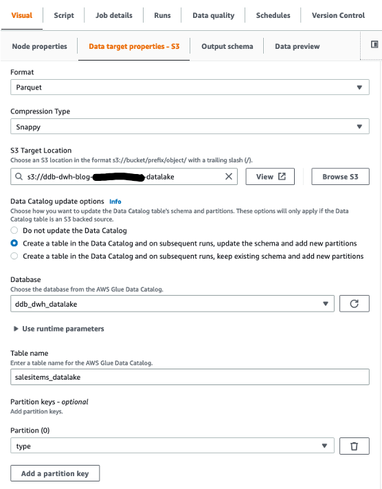
After the information is partitioned, we need to guarantee it’s held in the suitable format for optimum question efficiency. The beneficial selection is to make use of a columnar format reminiscent of Parquet or ORC. Such codecs are compressed and retailer information column-wise, permitting for quick retrieval occasions, and are parallelizable, permitting for quick load occasions when transferring the information into Amazon Redshift. In our use case, it is sensible to retailer the information in an information lake with minimal transformation and formatting to allow straightforward querying and exploration of the dataset. We partition the information by merchandise kind (Buyer, Order, Product, and so forth), and since we need to simply question every entity in an effort to transfer the information into our information warehouse, we remodel the information into the Parquet format.

Answer overview

The next diagram illustrates the information circulation to export information from a DynamoDB desk to an information warehouse.

We current a batch ELT answer utilizing AWS Glue for exporting information saved in DynamoDB to an Amazon Easy Storage Service (Amazon S3) information lake after which an information warehouse inbuilt Amazon Redshift. AWS Glue is a completely managed extract, remodel, and cargo (ETL) service that means that you can manage, cleanse, validate, and format information for storage in an information warehouse or information lake.

The answer workflow has the next steps:

1. Transfer any current recordsdata from the uncooked and information lake buckets into corresponding archive buckets to make sure any contemporary export from DynamoDB to Amazon S3 isn’t duplicating information.
2. Start a brand new DynamoDB export to the S3 uncooked layer.
3. From the uncooked recordsdata, create an information lake partitioned by merchandise kind.
4. Load the information from the information lake to touchdown tables in Amazon Redshift.
5. After the information is loaded, we benefit from the distributed compute functionality of Amazon Redshift to remodel the information into our dimensional mannequin and populate the information warehouse.

We orchestrate the pipeline utilizing an AWS Step Features workflow and schedule a day by day batch run utilizing Amazon EventBridge.

For easier DynamoDB desk constructions you could think about skipping a few of these steps by both loading information instantly from DynamoDB to Redshift or utilizing Redshift’s auto-copy or copy command to load information from S3.

Conditions

You could have an AWS account with a person who has programmatic entry. For setup directions, seek advice from AWS safety credentials.

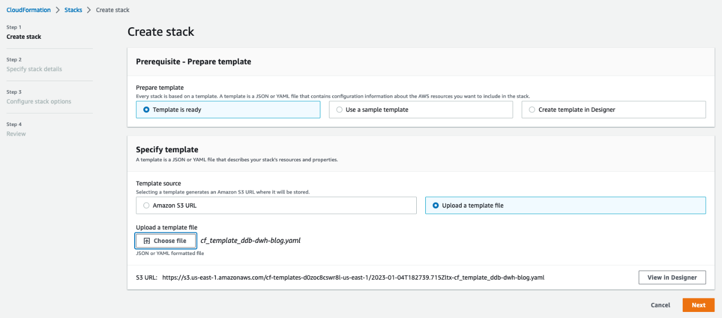
Use the AWS CloudFormation template cf_template_ddb-dwh-blog.yaml to launch the next assets:

• A DynamoDB desk with a GSI and point-in-time restoration enabled.
• An Amazon Redshift cluster (we use two nodes of RA3.4xlarge).
• Three AWS Glue database catalogs: uncooked, datalake, and redshift.
• 5 S3 buckets: two for the uncooked and information lake recordsdata; two for his or her respective archives, and one for the Amazon Athena question outcomes.
• Two AWS Identification and Entry Administration (IAM) roles: An AWS Glue function and a Step Features function with the requisite permissions and entry to assets.
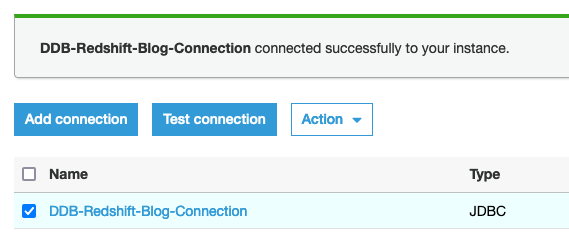
• A JDBC connection to Amazon Redshift.
• An AWS Lambda perform to retrieve the s3-prefix-list-id on your Area. That is required to permit site visitors from a VPC to entry an AWS service by a gateway VPC endpoint.
• Obtain the next recordsdata to carry out the ELT:
  • The Python script to load pattern information into our DynamoDB desk: load_dynamodb.py.
  • The AWS Glue Python Spark script to archive the uncooked and information lake recordsdata: archive_job.py.
  • The AWS Glue Spark scripts to extract and cargo the information from DynamoDB to Amazon Redshift: GlueSparkJobs.zip.
  • The DDL and DML SQL scripts to create the tables and cargo the information into the information warehouse in Amazon Redshift: SQL Scripts.zip.

Launch the CloudFormation template

AWS CloudFormation means that you can mannequin, provision, and scale your AWS assets by treating infrastructure as code. We use the downloaded CloudFormation template to create a stack (with new assets).

1. On the AWS CloudFormation console, create a brand new stack and choose Template is prepared.
2. Add the stack and select Subsequent.

3. Enter a reputation on your stack.
4. For MasterUserPassword, enter a password.
5. Optionally, change the default names for the Amazon Redshift database, DynamoDB desk, and MasterUsername (in case these names are already in use).
6. Reviewed the small print and acknowledge that AWS CloudFormation could create IAM assets in your behalf.
7. Select Create stack.

Load pattern information right into a DynamoDB desk

To load your pattern information into DynamoDB, full the next steps:

1. Create an AWS Cloud9 setting with default settings.
2. Add the load DynamoDB Python script. From the AWS Cloud9 terminal, use the pip set up command to put in the next packages:
   1. boto3
   2. faker
   3. faker_commerce
   4. numpy
3. Within the Python script, change all placeholders (capital letters) with the suitable values and run the next command within the terminal:

This command masses the pattern information into our single DynamoDB desk.

Extract information from DynamoDB

To extract the information from DynamoDB to our S3 information lake, we use the brand new AWS Glue DynamoDB export connector. Not like the previous connector, the brand new model makes use of a snapshot of the DynamoDB desk and doesn’t devour learn capability models of your supply DynamoDB desk. For big DynamoDB tables exceeding 100 GB, the learn efficiency of the brand new AWS Glue DynamoDB export connector will not be solely constant but additionally considerably quicker than the earlier model.

To make use of this new export connector, it’s essential allow point-in-time restoration (PITR) for the supply DynamoDB desk prematurely. This can take steady backups of the supply desk (so be conscious of price) and ensures that every time the connector invokes an export, the information is contemporary. The time it takes to finish an export will depend on the dimensions of your desk and the way uniformly the information is distributed therein. This may vary from a couple of minutes for small tables (as much as 10 GiB) to a couple hours for bigger tables (up to a couple terabytes). This isn’t a priority for our use case as a result of information lakes and information warehouses are sometimes used to mixture information at scale and generate day by day, weekly, or month-to-month reviews. It’s additionally value noting that every export is a full refresh of the information, so in an effort to construct a scalable automated information pipeline, we have to archive the present recordsdata earlier than starting a contemporary export from DynamoDB.

Full the next steps:

1. Create an AWS Glue job utilizing the Spark script editor.
2. Add the archive_job.py file from GlueSparkJobs.zip.

This job archives the information recordsdata into timestamped folders. We run the job concurrently to archive the uncooked recordsdata and the information lake recordsdata.

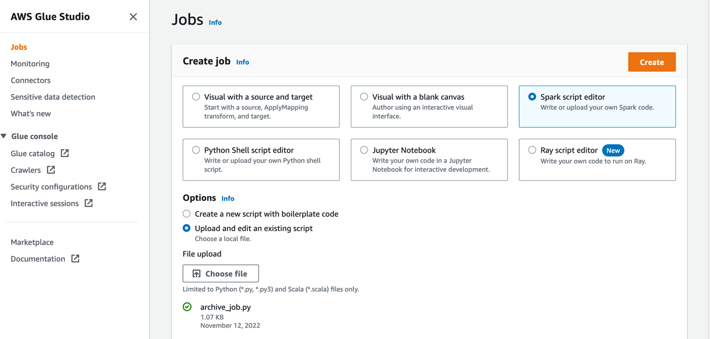
3. In Job particulars part, give the job a reputation and select the AWS Glue IAM function created by our CloudFormation template.
4. Maintain all defaults the identical and guarantee most concurrency is about to 2 (beneath Superior properties).

Archiving the recordsdata supplies a backup choice within the occasion of catastrophe restoration. As such, we are able to assume that the recordsdata is not going to be accessed incessantly and might be saved in Standard_IA storage class in order to avoid wasting as much as 40% on prices whereas offering speedy entry to the recordsdata when wanted.

This job sometimes runs earlier than every export of information from DynamoDB. After the datasets have been archived, we’re able to (re)-export the information from our DynamoDB desk.

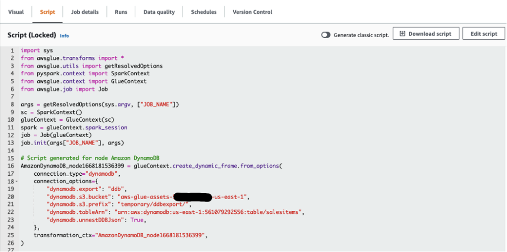
We will use AWS Glue Studio to visually create the roles wanted to extract the information from DynamoDB and cargo into our Amazon Redshift information warehouse. We show how to do that by creating an AWS Glue job (known as ddb_export_raw_job) utilizing AWS Glue Studio.

5. In AWS Glue Studio, create a job and choose Visible with a clean canvas.
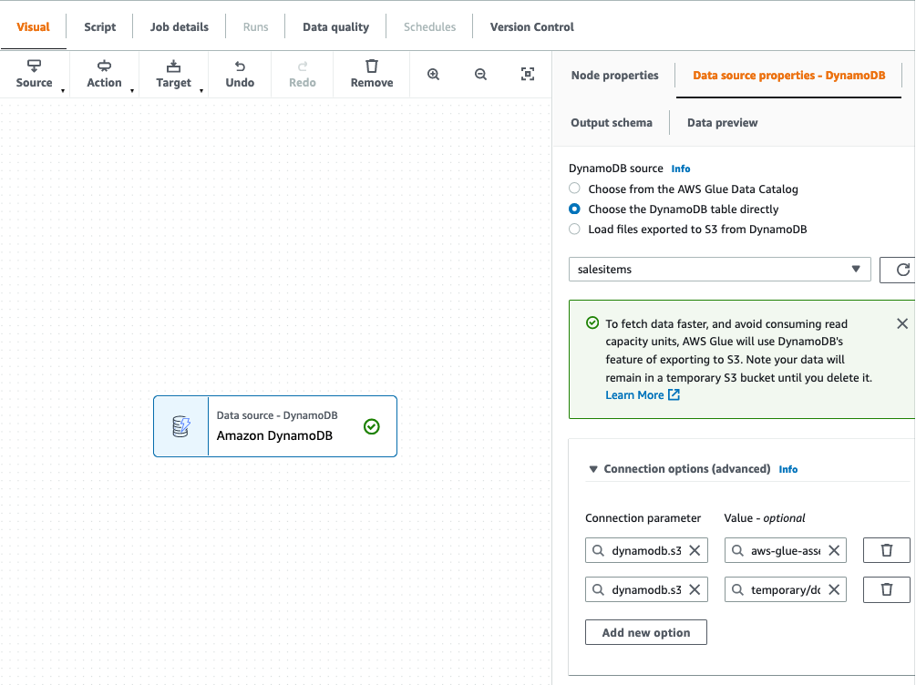
6. Select Amazon DynamoDB as the information supply.

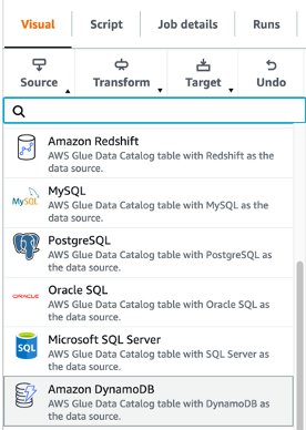
7. Select our DynamoDB desk to export from.
8. Go away all different choices as is and end organising the supply connection.

We then select Amazon S3 as our goal. Within the goal properties, we are able to remodel the output to an appropriate format, apply compression, and specify the S3 location to retailer our uncooked information.

9. Set the next choices:
   1. For Format, select Parquet.
   2. For Compression kind, select Snappy.
   3. For S3 Goal Location, enter the trail for RawBucket (positioned on the Outputs tab of the CloudFormation stack).
   4. For Database, select the worth for GlueRawDatabase (from the CloudFormation stack output).
   5. For Desk identify, enter an acceptable identify.

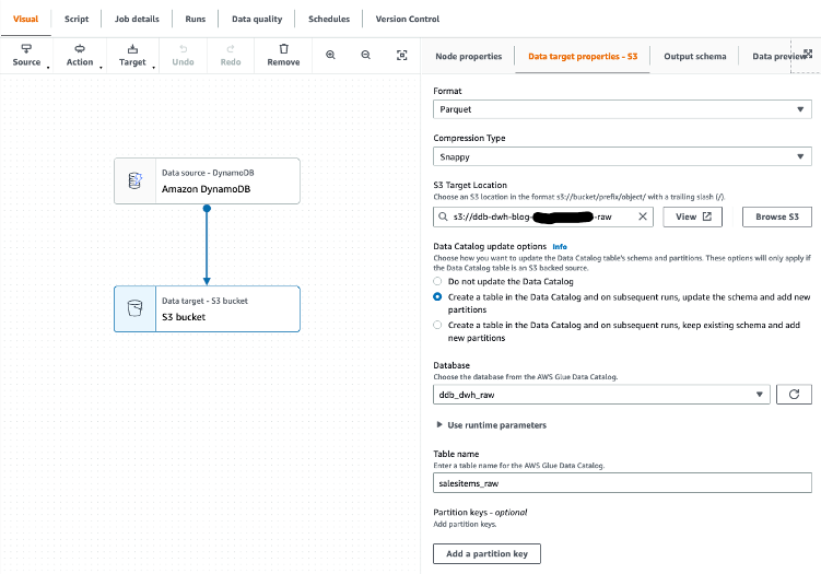
10. As a result of our goal information warehouse requires information to be in a flat construction, confirm that the configuration choice dynamodb.unnestDDBJson is about to True on the Script tab.

11. On the Job particulars tab, select the AWS Glue IAM function generated by the CloudFormation template.
12. Save and run the job.

Relying on the information volumes being exported, this job could take a couple of minutes to finish.

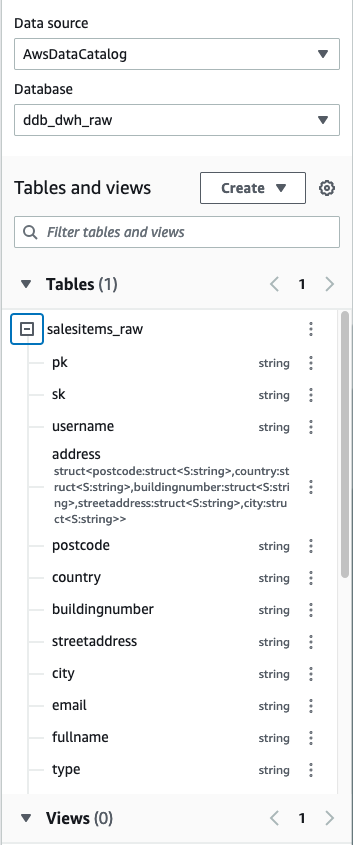
As a result of we’ll be including the desk to our AWS Glue Knowledge Catalog, we are able to discover the output utilizing Athena after the job is full. Athena is a serverless interactive question service that makes it easy to investigate information instantly in Amazon S3 utilizing normal SQL.

13. Within the Athena question editor, select the uncooked database.

We will see that the attributes of the Deal with construction have been unnested and added as extra columns to the desk.

14. After we export the information into the uncooked bucket, create one other job (known as raw_to_datalake_job) utilizing AWS Glue Studio (choose Visible with a clean canvas) to load the information lake partitioned by merchandise kind (buyer, order, and product).
15. Set the supply because the AWS Glue Knowledge Catalog uncooked database and desk.

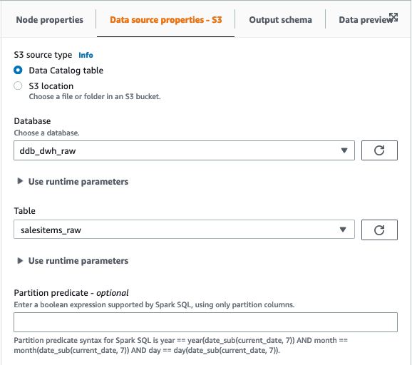
16. Within the ApplyMapping transformation, drop the Deal with struct as a result of we’ve already unnested these attributes into our flattened uncooked desk.

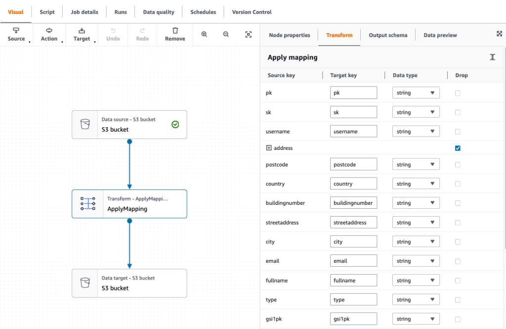
17. Set the goal as our S3 information lake.

18. Select the AWS Glue IAM function within the job particulars, then save and run the job.

Now that we’ve our information lake, we’re able to construct our information warehouse.

Construct the dimensional mannequin in Amazon Redshift

The CloudFormation template launches a two-node RA3.4xlarge Amazon Redshift cluster. To construct the dimensional mannequin, full the next steps:

1. In Amazon Redshift Question Editor V2, connect with your database (default: salesdwh) inside the cluster utilizing the database person identify and password authentication (MasterUserName and MasterUserPassword from the CloudFormation template).
2. Chances are you’ll be requested to configure your account if that is your first time utilizing Question Editor V2.
3. Obtain the SQL scripts SQL Scripts.zip to create the next schemas and tables (run the scripts in numbered sequence).

Within the touchdown schema:

• deal with
• buyer
• order
• product

Within the staging schema:

• staging.deal with
• staging.address_maxkey
• staging.addresskey
• staging.buyer
• staging.customer_maxkey
• staging.customerkey
• staging.date
• staging.date_maxkey
• staging.datekey
• staging.order
• staging.order_maxkey
• staging.orderkey
• staging.product
• staging.product_maxkey
• staging.productkey

Within the dwh schema:

• dwh.deal with
• dwh.buyer
• dwh.order
• dwh.product

We load the information from our information lake to the touchdown schema as is.

4. Use the JDBC connector to Amazon Redshift to construct an AWS Glue crawler so as to add the touchdown schema to our Knowledge Catalog beneath the ddb_redshift database.

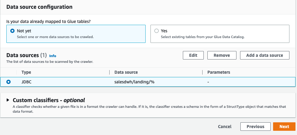
5. Create an AWS Glue crawler with the JDBC information supply.

6. Choose the JDBC connection you created and select Subsequent.

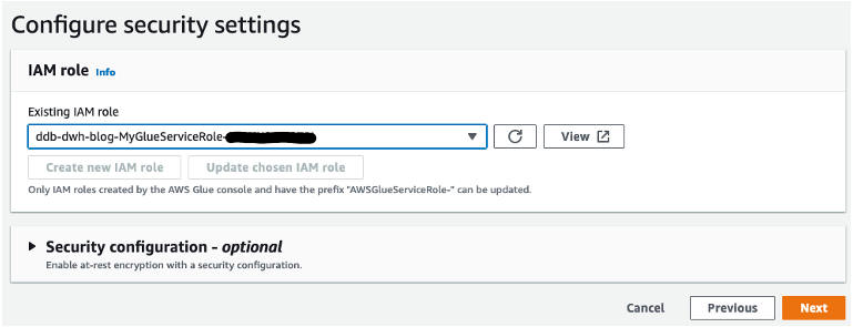
7. Select the IAM function created by the CloudFormation template and select Subsequent.

8. Evaluation your settings earlier than creating the crawler.

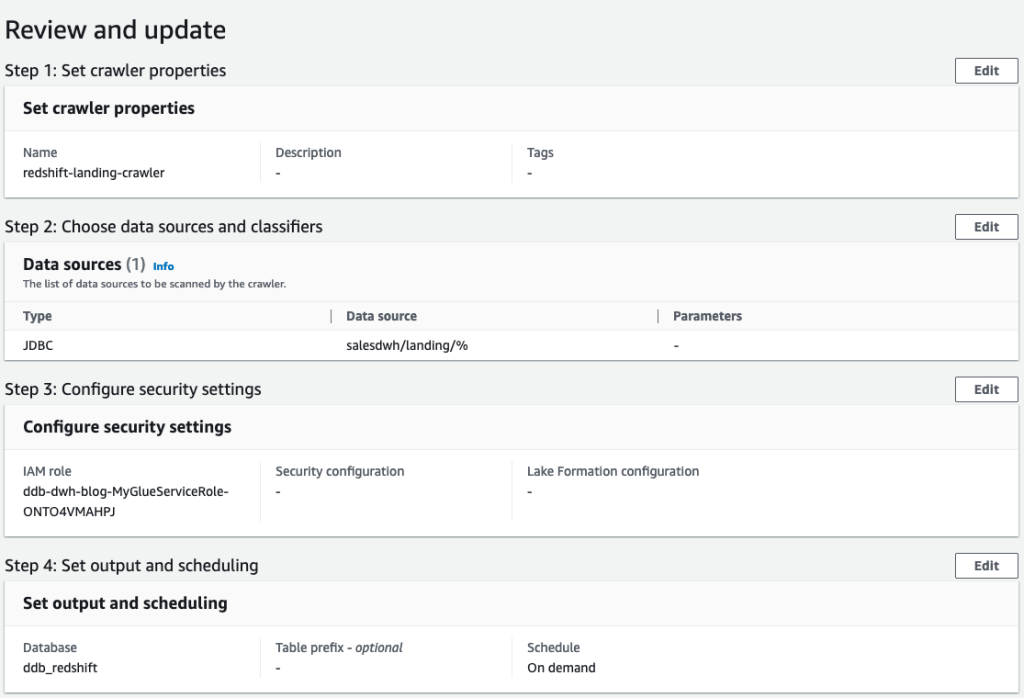
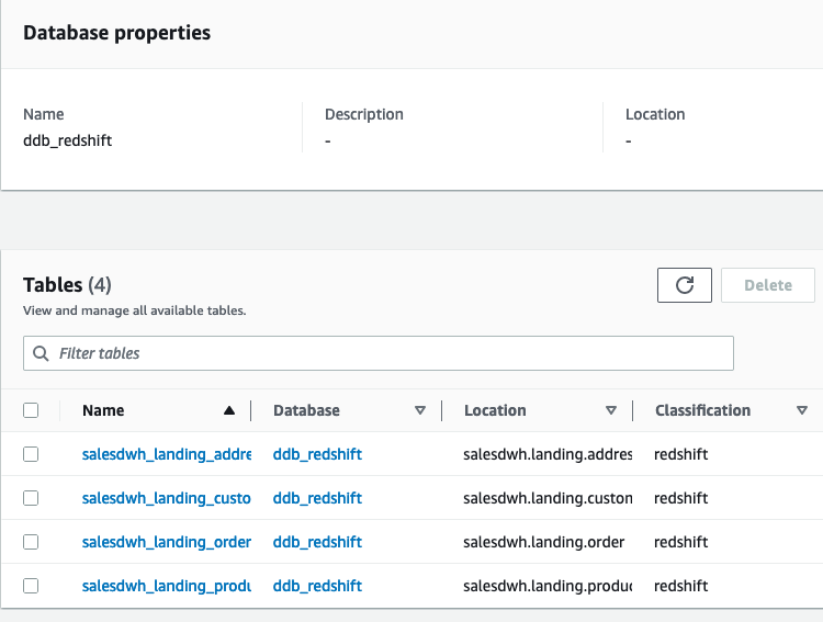
The crawler provides the 4 touchdown tables in our AWS Glue database ddb_redshift.

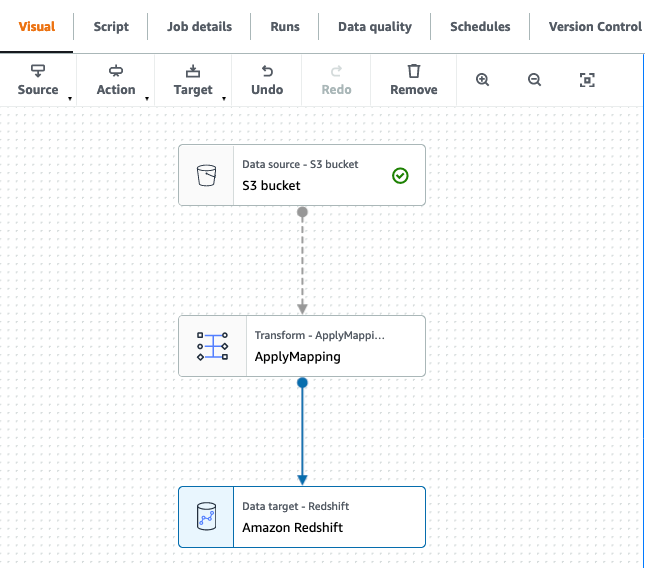
9. In AWS Glue Studio, create 4 AWS Glue jobs to load the touchdown tables (these scripts can be found to obtain, and you should use the Spark script editor to add these scripts individually to create the roles):
   1. land_order_job
   2. land_product_job
   3. land_customer_job
   4. land_address_job

Every job has the construction as proven within the following screenshot.

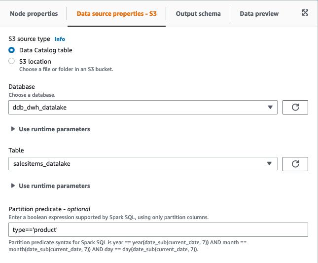
10. Filter the S3 supply on the partition column kind:
    1. For product, filter on kind=‘product’.
    2. For order, filter on kind=‘order’.
    3. For buyer and deal with, filter on kind=‘buyer’.

11. Set the goal for the information circulation because the corresponding desk within the touchdown schema in Amazon Redshift.
12. Use the built-in ApplyMapping transformation in our information pipeline to drop columns and, the place needed, convert the information sorts to match the goal columns.

For extra details about built-in transforms accessible in AWS Glue, seek advice from AWS Glue PySpark transforms reference.

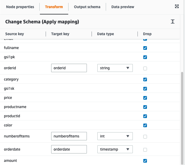
The mappings for our 4 jobs are as follows:

• land_order_job:

  mappings=[
  ("pk", "string", "pk", "string"),
  ("orderid", "string", "orderid", "string"),
  ("numberofitems", "string", "numberofitems", "int"),
  ("orderdate", "string", "orderdate", "timestamp"),
  ]

• land_product_job:

  mappings=[
  ("orderid", "string", "orderid", "string"),
  ("category", "string", "category", "string"),
  ("price", "string", "price", "decimal"),
  ("productname", "string", "productname", "string"),
  ("productid", "string", "productid", "string"),
  ("color", "string", "color", "string"),
  ]

• land_address_job:

  mappings=[
  ("username", "string", "username", "string"),
  ("email", "string", "email", "string"),
  ("fullname", "string", "fullname", "string"),
  ]

• land_customer_job:

  mappings=[
  ("username", "string", "username", "string"),
  ("email", "string", "email", "string"),
  ("fullname", "string", "fullname", "string"),
  ]

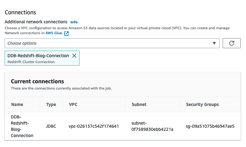
13. Select the AWS Glue IAM function, and beneath Superior properties, confirm the JDBC connector to Amazon Redshift as a connection.
14. Save and run every job to load the touchdown tables in Amazon Redshift.

Populate the information warehouse

From the touchdown schema, we transfer the information to the staging layer and apply the required transformations. Our dimensional mannequin has a single truth desk, the orders desk, which is the most important desk and as such wants a distribution key. The selection of key will depend on how the information is queried and the dimensions of the dimension tables being joined to. Should you’re uncertain of your question patterns, you’ll be able to go away the distribution keys and type keys on your tables unspecified. Amazon Redshift robotically assigns the right distribution and type keys primarily based in your queries. This has the benefit that if and when question patterns change over time, Amazon Redshift can robotically replace the keys to mirror the change in utilization.

Within the staging schema, we hold monitor of current information primarily based on their enterprise key (the distinctive identifier for the document). We create key tables to generate a numeric id column for every desk primarily based on the enterprise key. These key tables enable us to implement an incremental transformation of the information into our dimensional mannequin.

CREATE TABLE IF NOT EXISTS staging.productkey ( 
    productkey integer id(1,1), 
    productid character various(16383), 
    CONSTRAINT products_pkey PRIMARY KEY(productkey));   

When loading the information, we have to hold monitor of the most recent surrogate key worth to make sure that new information are assigned the right increment. We do that utilizing maxkey tables (pre-populated with zero):

CREATE TABLE IF NOT EXISTS staging.product_maxkey ( 
    productmaxkey integer);

INSERT INTO staging.product_maxkey
choose 0;    

We use staging tables to retailer our incremental load, the construction of which is able to mirror our last goal mannequin within the dwh schema:

---staging tables to load information from information lake 
   
CREATE TABLE IF NOT EXISTS staging.product ( 
    productkey integer,
    productname character various(200), 
    shade character various(50), 
    class character various(100),
    PRIMARY KEY (productkey));

---dwh tables to load information from staging schema
     
CREATE TABLE IF NOT EXISTS dwh.product ( 
    productkey integer,
    productname character various(200), 
    shade character various(50), 
    class character various(100),
    PRIMARY KEY (productkey)); 

Incremental processing within the information warehouse

We load the goal information warehouse utilizing saved procedures to carry out upserts (deletes and inserts carried out in a single transaction):

CREATE OR REPLACE PROCEDURE staging.load_order() LANGUAGE plpgsql AS $$
DECLARE
BEGIN

TRUNCATE TABLE staging.order;

--insert new information to get new ids
insert into staging.orderkey
(
orderid
)
choose
c.orderid
from touchdown.order c
LEFT JOIN staging.orderkey i
ON c.orderid=i.orderid
the place i.orderid IS NULL;

--update the max key
replace staging.order_maxkey
set ordermaxkey = (choose max(orderkey) from staging.orderkey);


insert into staging.order
(
orderkey,
customerkey,
productkey,
addresskey,
datekey,
numberofitems,
worth
)
choose
xid.orderkey,
cid.customerkey,
pid.productkey,
assist.addresskey,
d.datekey,
o.numberofitems,
p.worth
from
touchdown.order o
be a part of staging.orderkey xid on o.orderid=xid.orderid
be a part of touchdown.buyer c on substring(o.pk,6,size(o.pk))=c.username   ---order desk wants username
be a part of staging.customerkey cid on cid.username=c.username
be a part of touchdown.deal with a on a.username=c.username
be a part of staging.addresskey assist on assist.pk=a.buildingnumber::varchar+'||'+a.postcode  ---maybe change pk to addressid
be a part of staging.datekey d on d.orderdate=o.orderdate
be a part of touchdown.product p on p.orderid=o.orderid
be a part of staging.productkey pid on pid.productid=p.productid;

COMMIT;

END;
$$ 

CREATE OR REPLACE PROCEDURE dwh.load_order() LANGUAGE plpgsql AS $$
DECLARE
BEGIN

---delete previous information 
delete from dwh.order
utilizing staging.order as stage
the place dwh.order.orderkey=stage.orderkey;

--insert new and modified
insert into dwh.order
(
orderkey,
customerkey,  
productkey,
addresskey,
worth,
datekey  
)
choose
orderkey,
customerkey,  
productkey,
addresskey,
worth,
datekey
from staging.order;

COMMIT;
END;
$$

Use Step Features to orchestrate the information pipeline

To this point, we’ve stepped by every element in our workflow. We now must sew them collectively to construct an automatic, idempotent information pipeline. A great orchestration device should handle failures, retries, parallelization, service integrations, and observability, so builders can focus solely on the enterprise logic. Ideally, the workflow we construct can be serverless so there isn’t a operational overhead. Step Features is a perfect option to automate our information pipeline. It permits us to combine the ELT parts we’ve constructed on AWS Glue and Amazon Redshift and conduct some steps in parallel to optimize efficiency.

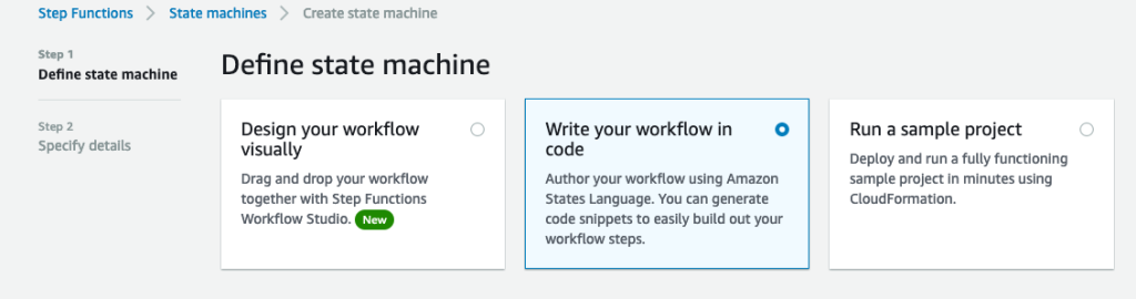
1. On the Step Features console, create a brand new state machine.
2. Choose Write your workflow in code.

3. Enter the stepfunction_workflow.json code into the definition, changing all placeholders with the suitable values:
   1. [REDSHIFT-CLUSTER-IDENTIFIER] – Use the worth for ClusterName (from the Outputs tab within the CloudFormation stack).
   2. [REDSHIFT-DATABASE] – Use the worth for salesdwh (except modified, that is the default database within the CloudFormation template).

We use the Step Features IAM function from the CloudFormation template.

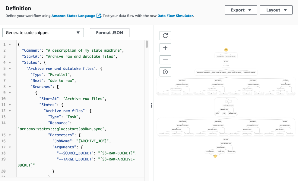
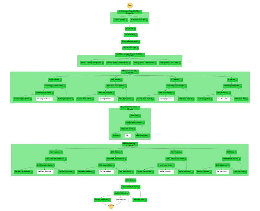
This JSON code generates the next pipeline.

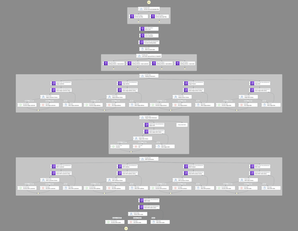
Ranging from the highest, the workflow incorporates the next steps:

1. We archive any current uncooked and information lake recordsdata.
2. We add two AWS Glue StartJobRun duties that run sequentially: first to export the information from DynamoDB to our uncooked bucket, then from the uncooked bucket to our information lake.
3. After that, we parallelize the touchdown of information from Amazon S3 to Amazon Redshift.
4. We remodel and cargo the information into our information warehouse utilizing the Amazon Redshift Knowledge API. As a result of that is asynchronous, we have to examine the standing of the runs earlier than transferring down the pipeline.
5. After we transfer the information load from touchdown to staging, we truncate the touchdown tables.
6. We load the scale of our goal information warehouse (dwh) first, and eventually we load our single truth desk with its overseas key dependency on the previous dimension tables.

The next determine illustrates a profitable run.

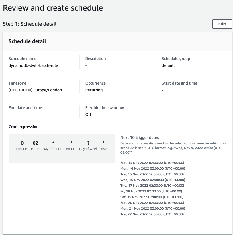
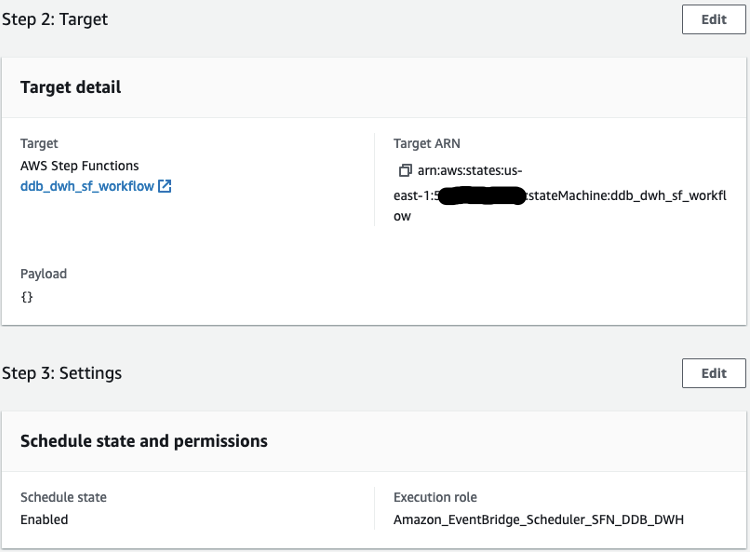
After we arrange the workflow, we are able to use EventBridge to schedule a day by day midnight run, the place the goal is a Step Features StartExecution API calling our state machine. Underneath the workflow permissions, select Create a brand new function for this schedule and optionally rename it.

Question the information warehouse

We will confirm the information has been efficiently loaded into Amazon Redshift with a question.

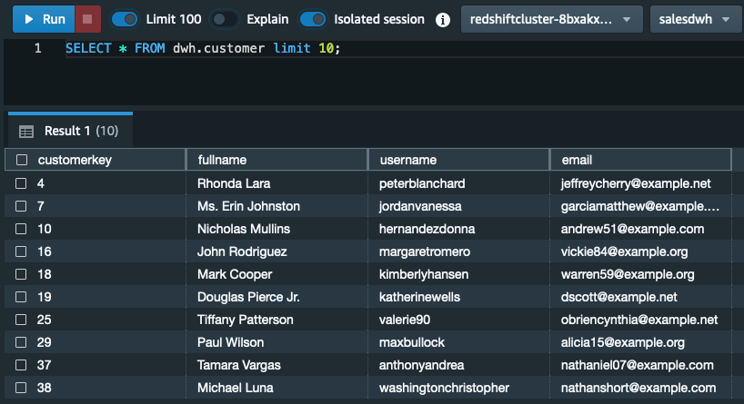
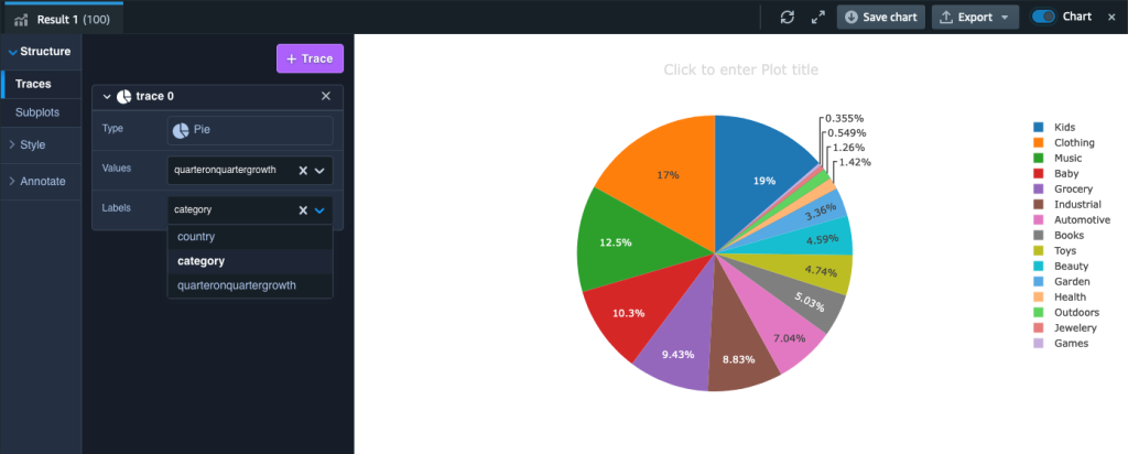
After we’ve the information loaded into Amazon Redshift, we’re able to reply the question requested at the beginning of this submit: what’s the year-on-year quarterly gross sales development by product and nation? The question appears like the next code (relying in your dataset, you could want to pick different years and quarters):

with sales2021q2
as
(
  choose d.12 months, d.quarter,a.nation,p.class,sum(o.worth) as revenue2021q2
  from dwh.order o
  be a part of dwh.date d on o.datekey=d.datekey
  be a part of dwh.product p on o.productkey=p.productkey
  be a part of dwh.deal with a on a.addresskey=o.addresskey
  the place d.12 months=2021 and d.quarter=2
  group by d.12 months, d.quarter,a.nation,p.class
  ),
sales2022q2
as
(
  choose d.12 months, d.quarter,a.nation,p.class,sum(o.worth) as revenue2022q2
  from dwh.order o
  be a part of dwh.date d on o.datekey=d.datekey
  be a part of dwh.product p on o.productkey=p.productkey
  be a part of dwh.deal with a on a.addresskey=o.addresskey
  the place d.12 months=2022 and d.quarter=2
  group by d.12 months, d.quarter,a.nation,p.class
  )

choose a.nation,a.class, ((revenue2022q2 - revenue2021q2)/revenue2021q2)*100 as quarteronquartergrowth
from sales2022q2 a
be a part of sales2021q2 b on a.nation=b.nation and a.class=b.class
order by a.nation,a.class

We will visualize the ends in Amazon Redshift Question Editor V2 by toggling the chart choice and setting Sort as Pie, Values as quarteronquartergrowth, and Labels as class.

Value concerns

We give a short define of the indicative prices related to the important thing companies coated in our answer primarily based on us-east-1 Area pricing utilizing the AWS Pricing Calculator:

• DynamoDB – With on-demand settings for 1.5 million gadgets (common measurement of 355 bytes) and related write and browse capability plus PITR storage, the price of DynamoDB is roughly $2 per thirty days.
• AWS Glue DynamoDB export connector – This connector makes use of the DynamoDB export to Amazon S3 characteristic. This has no hourly price—you solely pay for the gigabytes of information exported to Amazon S3 ($0.11 per GiB).
• Amazon S3 – You pay for storing objects in your S3 buckets. The speed you’re charged will depend on your objects’ measurement, how lengthy you saved the objects throughout the month, and the storage class. In our answer, we used S3 Commonplace for our information lake and S3 Commonplace – Rare Entry for archive. Commonplace-IA storage is $0.0125 per GB/month; Commonplace storage is $0.023 per GB/month.
• AWS Glue Jobs – With AWS Glue, you solely pay for the time your ETL job takes to run. There aren’t any assets to handle, no upfront prices, and you aren’t charged for startup or shutdown time. AWS costs you an hourly price primarily based on the variety of Knowledge Processing Items (DPUs) used to run your ETL job. A single DPU supplies 4 vCPU and 16 GB of reminiscence. Each considered one of our 9 Spark jobs makes use of 10 DPUs and has a mean runtime of three minutes. This offers an approximate price of $0.29 per job.
• Amazon Redshift – We provisioned two RA3.4xlarge nodes for our Amazon Redshift cluster. If run on-demand, every node prices $3.26 per hour. If utilized 24/7, our month-to-month price could be roughly $4,759.60. You must consider your workload to find out what price financial savings might be achieved by utilizing Amazon Redshift Serverless or utilizing Amazon Redshift provisioned reserved cases.
• Step Features – You might be charged primarily based on the variety of state transitions required to run your utility. Step Features counts a state transition as every time a step of your workflow is run. You’re charged for the entire variety of state transitions throughout all of your state machines, together with retries. The Step Features free tier contains 4,000 free state transitions per thirty days. Thereafter, it’s $0.025 per 1,000 state transitions.

Clear up

Keep in mind to delete any assets created by the CloudFormation stack. You first must manually empty and delete the S3 buckets. Then you’ll be able to delete the CloudFormation stack utilizing the AWS CloudFormation console or AWS Command Line Interface (AWS CLI). For directions, seek advice from Clear up your “good day, world!” utility and associated assets.

Abstract

On this submit, we demonstrated how one can export information from DynamoDB to Amazon S3 and Amazon Redshift to carry out superior analytics. We constructed an automatic information pipeline that you should use to carry out a batch ELT course of that may be scheduled to run day by day, weekly, or month-to-month and might scale to deal with very massive workloads.

Please go away your suggestions or feedback within the feedback part.

In regards to the Creator

Altaf Hussain is an Analytics Specialist Options Architect at AWS. He helps prospects across the globe design and optimize their large information and information warehousing options.

Appendix

To extract the information from DynamoDB and cargo it into our Amazon Redshift database, we are able to use the Spark script editor and add the recordsdata from GlueSparkJobs.zip to create every particular person job essential to carry out the extract and cargo. Should you select to do that, bear in mind to replace, the place acceptable, the account ID and Area placeholders within the scripts. Additionally, on the Job particulars tab beneath Superior properties, add the Amazon Redshift connection.