

The rubbish collector is a fancy piece of equipment that may be tough to tune. Certainly, the G1 collector alone has over 20 tuning flags. Not surprisingly, many builders dread touching the GC. Should you don’t give the GC just a bit little bit of care, your entire software is likely to be operating suboptimal. So, what if we let you know that tuning the GC doesn’t must be onerous? Actually, simply by following a easy recipe, your GC and your entire software might already get a efficiency increase.
This weblog submit exhibits how we obtained two manufacturing purposes to carry out higher by following easy tuning steps. In what follows, we present you the way we gained a two instances higher throughput for a streaming software. We additionally present an instance of a misconfigured high-load, low-latency REST service with an abundantly giant heap. By taking some easy steps, we diminished the heap dimension greater than ten-fold with out compromising latency. Earlier than we achieve this, we’ll first clarify the recipe we adopted that spiced up our purposes’ efficiency.
A easy recipe for GC tuning
Let’s begin with the substances of our recipe:
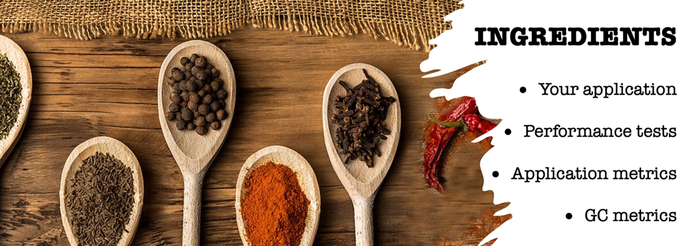
Moreover your software that wants spicing, you need some strategy to generate a production-like load on a check atmosphere – except feeling courageous sufficient to make performance-impacting modifications in your manufacturing atmosphere.
To guage how good your app does, you want some metrics on its key efficiency indicators. Which metrics rely upon the precise objectives of your software. For instance, latency for a service and throughput for a streaming software. Moreover these metrics, you additionally need details about how a lot reminiscence your app consumes. We use Micrometer to seize our metrics, Prometheus to extract them, and Grafana to visualise them.
Along with your app metrics, your key efficiency indicators are coated, however in the long run, it’s the GC we like to boost. Except being eager about hardcore GC tuning, these are the three key efficiency indicators to find out how good of a job your GC is doing:
- Latency – how lengthy does a single rubbish accumulating occasion pause your software.
- Throughput – how a lot time does your software spend on rubbish accumulating, and the way a lot time can it spend on doing software work.
- Footprint – the CPU and reminiscence utilized by the GC to carry out its job
This final ingredient, the GC metrics, is likely to be a bit tougher to seek out. Micrometer exposes them. (See for instance this weblog submit for an summary of metrics.) Alternatively, you can receive them out of your software’s GC logs. (You’ll be able to seek advice from this text to learn to receive and analyze them.)
Now we’ve got all of the substances we’d like, it’s time for the recipe:
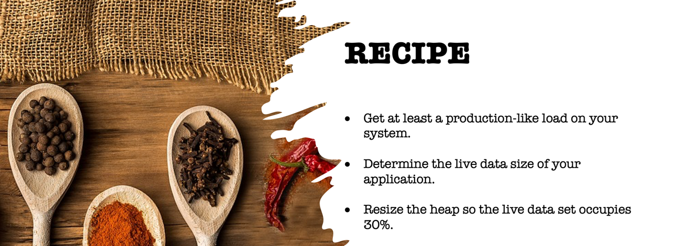
Let’s get cooking. Hearth up your efficiency exams and preserve them operating for a interval to heat up your software. At this level it’s good to put in writing down issues like response instances, most requests per second. This fashion, you possibly can evaluate completely different runs with completely different settings later.
Subsequent, you establish your app’s reside knowledge dimension (LDS). The LDS is the scale of all of the objects remaining after the GC collects all unreferenced objects. In different phrases, the LDS is the reminiscence of the objects your app nonetheless makes use of. With out going into an excessive amount of element, you have to:
- Set off a full rubbish accumulate, which forces the GC to gather all unused objects on the heap. You’ll be able to set off one from a profiler reminiscent of VisualVM or JDK Mission Management.
- Learn the used heap dimension after the total accumulate. Beneath regular circumstances it’s best to have the ability to simply acknowledge the total accumulate by the massive drop in reminiscence. That is the reside knowledge dimension.
The final step is to recalculate your software’s heap. Most often, your LDS ought to occupy round 30% of the heap (Java Efficiency by Scott Oaks). It’s good apply to set your minimal heap (Xms) equal to your most heap (Xmx). This prevents the GC from doing costly full collects on each resize of the heap. So, in a method: Xmx = Xms = max(LDS) / 0.3
Spicing up a streaming software
Think about you might have an software that processes messages which can be revealed on a queue. The appliance runs within the Google cloud and makes use of horizontal pod autoscaling to robotically scale the variety of software nodes to match the queue’s workload. Every little thing appears to run high-quality for months already, however does it?
The Google cloud makes use of a pay-per-use mannequin, so throwing in additional software nodes to spice up your software’s efficiency comes at a worth. So, we determined to check out our recipe on this software to see if there’s something to achieve right here. There actually was, so learn on.
Earlier than
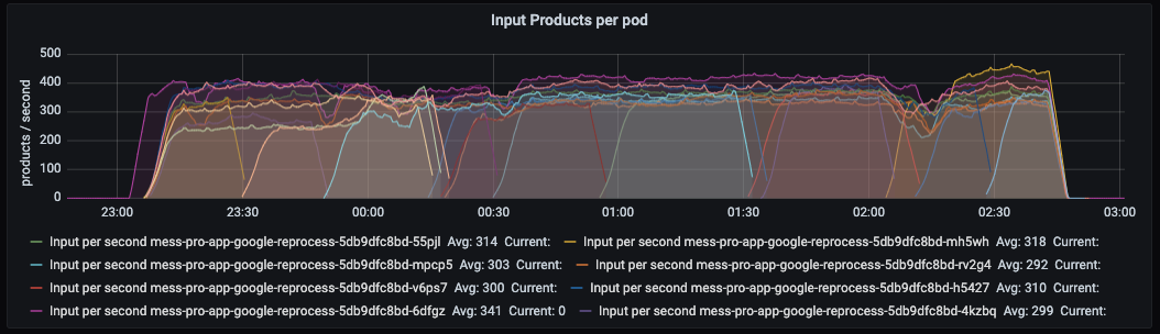
To determine a baseline, we ran a efficiency check to get insights into the appliance’s key efficiency metrics. We additionally downloaded the appliance’s GC logs to be taught extra about how the GC behaves. The beneath Grafana dashboard exhibits what number of parts (merchandise) every software node processes per second: max 200 on this case.
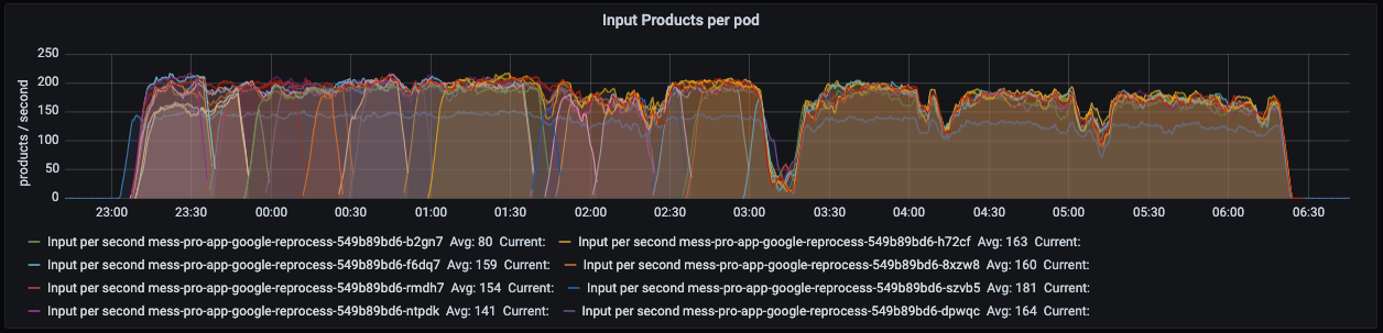
These are the volumes we’re used to, so all good. Nonetheless, whereas inspecting the GC logs, we discovered one thing that shocked us.

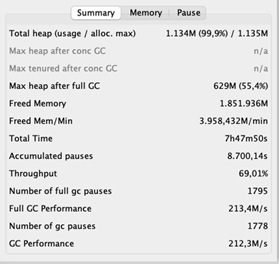
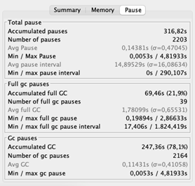
The typical pause time is 2,43 seconds. Recall that in pauses, the appliance is unresponsive. Lengthy delays don’t should be a problem for a streaming software as a result of it doesn’t have to answer shoppers’ requests. The stunning half is its throughput of 69%, which signifies that the appliance spends 31% of its time wiping out reminiscence. That’s 31% not being spent on area logic. Ideally, the throughput must be no less than 95%.
Figuring out the reside knowledge dimension
Allow us to see if we are able to make this higher. We decide the LDS by triggering a full rubbish accumulate whereas the appliance is beneath load. Our software was performing so dangerous that it already carried out full collects – this usually signifies that the GC is in bother. On the brilliant aspect, we do not have to set off a full accumulate manually to determine the LDS.
We distilled that the max heap dimension after a full GC is roughly 630MB. Making use of our rule of thumb yields a heap of 630 / 0.3 = 2100MB. That’s nearly twice the scale of our present heap of 1135MB!
After
Inquisitive about what this might do to our software, we elevated the heap to 2100MB and fired up our efficiency exams as soon as extra. The outcomes excited us.

After growing the heap, the typical GC pauses decreased rather a lot. Additionally, the GC’s throughput improved dramatically – 99% of the time the appliance is doing what it’s supposed to do. And the throughput of the appliance, you ask? Recall that earlier than, the appliance processed 200 parts per second at most. Now it peaks at 400 per second!
Spicing up a high-load, low-latency REST service
Quiz query. You’ve gotten a low-latency, high-load service operating on 42 digital machines, every having 2 CPU cores. Sometime, you migrate your software nodes to 5 beasts of bodily servers, every having 32 CPU cores. Given that every digital machine had a heap of 2GB, what dimension ought to or not it’s for every bodily server?
So, you have to divide 42 * 2 = 84GB of whole reminiscence over 5 machines. That boils right down to 84 / 5 = 16.8GB per machine. To take no probabilities, you spherical this quantity as much as 25GB. Sounds believable, proper? Nicely, the right reply seems to be lower than 2GB, as a result of that’s the quantity we obtained by calculating the heap dimension based mostly on the LDS. Can’t consider it? No worries, we couldn’t consider it both. Due to this fact, we determined to run an experiment.
Experiment setup
We’ve 5 software nodes, so we are able to run our experiment with 5 differently-sized heaps. We give node one 2GB, node two 4GB, node three 8GB, node 4 12GB, and node 5 25GB. (Sure, we aren’t courageous sufficient to run our software with a heap beneath 2GB.)
As a subsequent step, we hearth up our efficiency exams producing a steady, production-like load of a baffling 56K requests per second. All through the entire run of this experiment, we measure the variety of requests every node receives to make sure that the load is equally balanced. What’s extra, we measure this service’s key efficiency indicator – latency.
As a result of we obtained weary of downloading the GC logs after every check, we invested in Grafana dashboards to indicate us the GC’s pause instances, throughput, and heap dimension after a rubbish accumulate. This fashion we are able to simply examine the GC’s well being.
Outcomes
This weblog is about GC tuning, so let’s begin with that. The next determine exhibits the GC’s pause instances and throughput. Recall that pause instances point out how lengthy the GC freezes the appliance whereas sweeping out reminiscence. Throughput then specifies the share of time the appliance shouldn’t be paused by the GC.
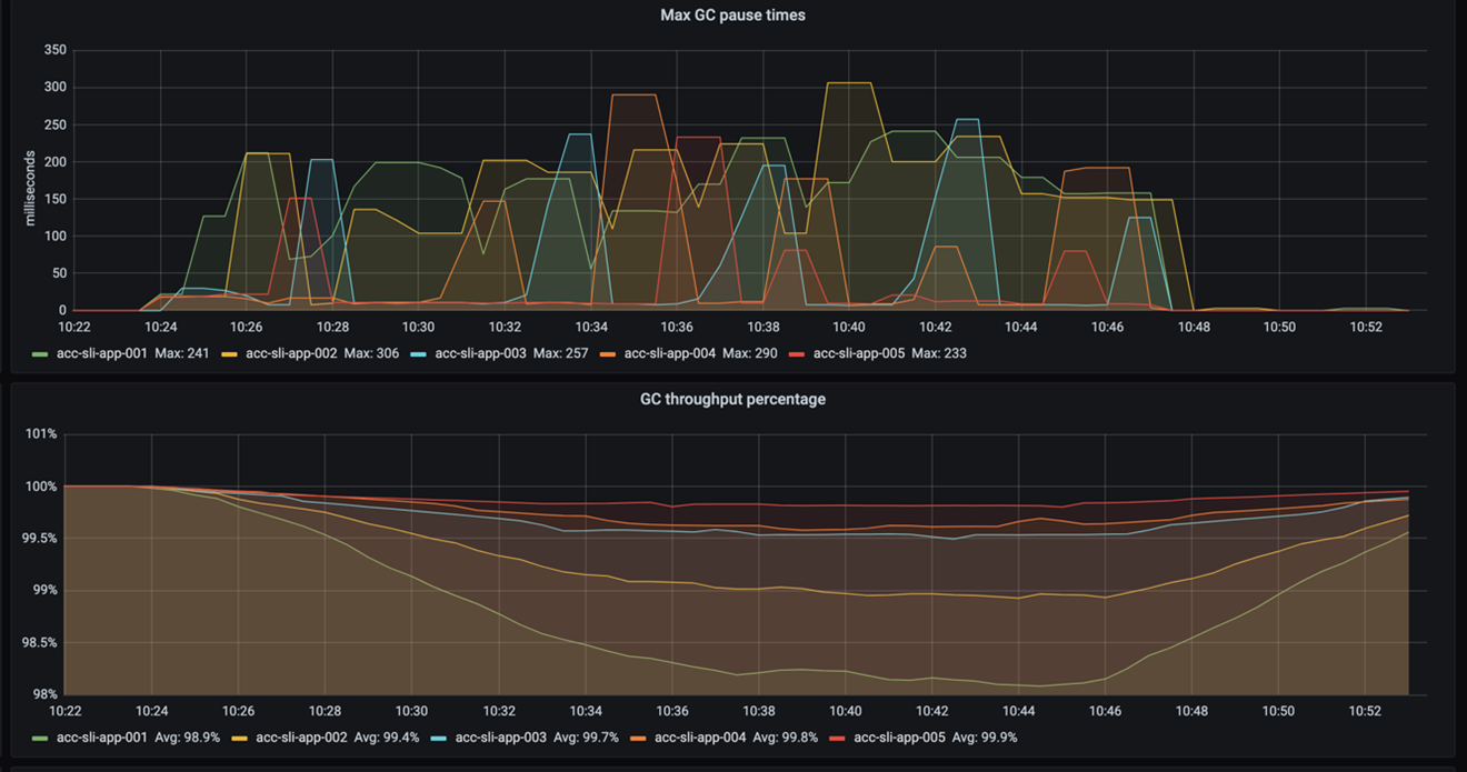
As you possibly can see, the pause frequency and pause instances don’t differ a lot. The throughput exhibits it greatest: the smaller the heap, the extra the GC pauses. It additionally exhibits that even with a 2GB heap the throughput remains to be OK – it doesn’t drop beneath 98%. (Recall {that a} throughput increased than 95% is taken into account good.)
So, growing a 2GB heap by 23GB will increase the throughput by nearly 2%. That makes us surprise, how vital is that for the general software’s efficiency? For the reply, we have to take a look at the appliance’s latency.
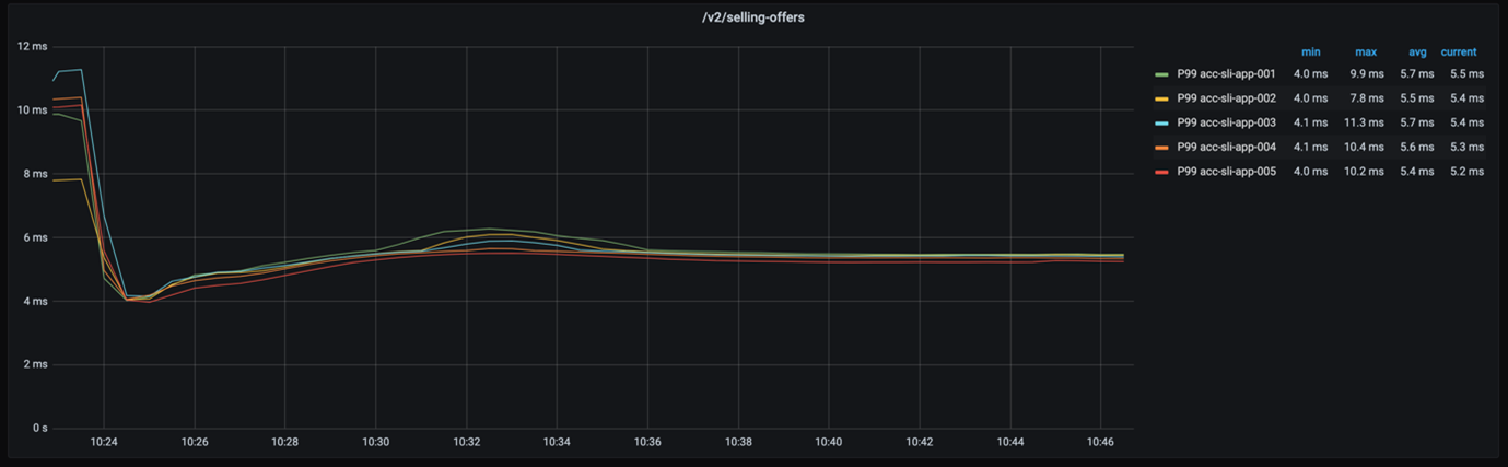
If we take a look at the 99-percentile latency of every node – as proven within the beneath graph – we see that the response instances are actually shut.
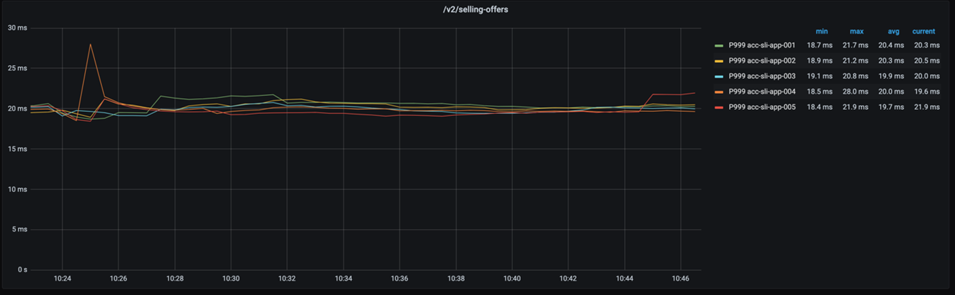
Even when we contemplate the 999-percentile, the response instances of every node are nonetheless not very far aside, as the next graph exhibits.
How does the drop of just about 2% in GC throughput have an effect on our software’s general efficiency? Not a lot. And that’s nice as a result of it means two issues. First, the easy recipe for GC tuning labored once more. Second, we simply saved a whopping 115GB of reminiscence!
Conclusion
We defined a easy recipe of GC tuning that served two purposes. By growing the heap, we gained two instances higher throughput for a streaming software. We diminished the reminiscence footprint of a REST service greater than ten-fold with out compromising its latency. All of that we achieved by following these steps:
• Run the appliance beneath load.
• Decide the reside knowledge dimension (the scale of the objects your software nonetheless makes use of).
• Dimension the heap such that the LDS takes 30% of the entire heap dimension.
Hopefully, we satisfied you that GC tuning does not should be daunting. So, deliver your personal substances and begin cooking. We hope the end result will likely be as spicy as ours.
Credit
Many due to Alexander Bolhuis, Ramin Gomari, Tomas Sirio and Deny Rubinskyi for serving to us run the experiments. We couldn’t have written this weblog submit with out you guys.